hypothesis testing for mean standard deviation unknown

Hypothesis Testing Calculator

Related: confidence interval calculator, type ii error.

The first step in hypothesis testing is to calculate the test statistic. The formula for the test statistic depends on whether the population standard deviation (σ) is known or unknown. If σ is known, our hypothesis test is known as a z test and we use the z distribution. If σ is unknown, our hypothesis test is known as a t test and we use the t distribution. Use of the t distribution relies on the degrees of freedom, which is equal to the sample size minus one. Furthermore, if the population standard deviation σ is unknown, the sample standard deviation s is used instead. To switch from σ known to σ unknown, click on $\boxed{\sigma}$ and select $\boxed{s}$ in the Hypothesis Testing Calculator.

Next, the test statistic is used to conduct the test using either the p-value approach or critical value approach. The particular steps taken in each approach largely depend on the form of the hypothesis test: lower tail, upper tail or two-tailed. The form can easily be identified by looking at the alternative hypothesis (H a ). If there is a less than sign in the alternative hypothesis then it is a lower tail test, greater than sign is an upper tail test and inequality is a two-tailed test. To switch from a lower tail test to an upper tail or two-tailed test, click on $\boxed{\geq}$ and select $\boxed{\leq}$ or $\boxed{=}$, respectively.

In the p-value approach, the test statistic is used to calculate a p-value. If the test is a lower tail test, the p-value is the probability of getting a value for the test statistic at least as small as the value from the sample. If the test is an upper tail test, the p-value is the probability of getting a value for the test statistic at least as large as the value from the sample. In a two-tailed test, the p-value is the probability of getting a value for the test statistic at least as unlikely as the value from the sample.

To test the hypothesis in the p-value approach, compare the p-value to the level of significance. If the p-value is less than or equal to the level of signifance, reject the null hypothesis. If the p-value is greater than the level of significance, do not reject the null hypothesis. This method remains unchanged regardless of whether it's a lower tail, upper tail or two-tailed test. To change the level of significance, click on $\boxed{.05}$. Note that if the test statistic is given, you can calculate the p-value from the test statistic by clicking on the switch symbol twice.

In the critical value approach, the level of significance ($\alpha$) is used to calculate the critical value. In a lower tail test, the critical value is the value of the test statistic providing an area of $\alpha$ in the lower tail of the sampling distribution of the test statistic. In an upper tail test, the critical value is the value of the test statistic providing an area of $\alpha$ in the upper tail of the sampling distribution of the test statistic. In a two-tailed test, the critical values are the values of the test statistic providing areas of $\alpha / 2$ in the lower and upper tail of the sampling distribution of the test statistic.

To test the hypothesis in the critical value approach, compare the critical value to the test statistic. Unlike the p-value approach, the method we use to decide whether to reject the null hypothesis depends on the form of the hypothesis test. In a lower tail test, if the test statistic is less than or equal to the critical value, reject the null hypothesis. In an upper tail test, if the test statistic is greater than or equal to the critical value, reject the null hypothesis. In a two-tailed test, if the test statistic is less than or equal the lower critical value or greater than or equal to the upper critical value, reject the null hypothesis.

When conducting a hypothesis test, there is always a chance that you come to the wrong conclusion. There are two types of errors you can make: Type I Error and Type II Error. A Type I Error is committed if you reject the null hypothesis when the null hypothesis is true. Ideally, we'd like to accept the null hypothesis when the null hypothesis is true. A Type II Error is committed if you accept the null hypothesis when the alternative hypothesis is true. Ideally, we'd like to reject the null hypothesis when the alternative hypothesis is true.

Hypothesis testing is closely related to the statistical area of confidence intervals. If the hypothesized value of the population mean is outside of the confidence interval, we can reject the null hypothesis. Confidence intervals can be found using the Confidence Interval Calculator . The calculator on this page does hypothesis tests for one population mean. Sometimes we're interest in hypothesis tests about two population means. These can be solved using the Two Population Calculator . The probability of a Type II Error can be calculated by clicking on the link at the bottom of the page.

Teach yourself statistics

Hypothesis Test for a Mean

This lesson explains how to conduct a hypothesis test of a mean, when the following conditions are met:

• The sampling method is simple random sampling .
• The sampling distribution is normal or nearly normal.

Generally, the sampling distribution will be approximately normally distributed if any of the following conditions apply.

• The population distribution is normal.
• The population distribution is symmetric , unimodal , without outliers , and the sample size is 15 or less.
• The population distribution is moderately skewed , unimodal, without outliers, and the sample size is between 16 and 40.
• The sample size is greater than 40, without outliers.

This approach consists of four steps: (1) state the hypotheses, (2) formulate an analysis plan, (3) analyze sample data, and (4) interpret results.

State the Hypotheses

Every hypothesis test requires the analyst to state a null hypothesis and an alternative hypothesis . The hypotheses are stated in such a way that they are mutually exclusive. That is, if one is true, the other must be false; and vice versa.

The table below shows three sets of hypotheses. Each makes a statement about how the population mean μ is related to a specified value M . (In the table, the symbol ≠ means " not equal to ".)

The first set of hypotheses (Set 1) is an example of a two-tailed test , since an extreme value on either side of the sampling distribution would cause a researcher to reject the null hypothesis. The other two sets of hypotheses (Sets 2 and 3) are one-tailed tests , since an extreme value on only one side of the sampling distribution would cause a researcher to reject the null hypothesis.

Formulate an Analysis Plan

The analysis plan describes how to use sample data to accept or reject the null hypothesis. It should specify the following elements.

• Significance level. Often, researchers choose significance levels equal to 0.01, 0.05, or 0.10; but any value between 0 and 1 can be used.
• Test method. Use the one-sample t-test to determine whether the hypothesized mean differs significantly from the observed sample mean.

Analyze Sample Data

Using sample data, conduct a one-sample t-test. This involves finding the standard error, degrees of freedom, test statistic, and the P-value associated with the test statistic.

SE = s * sqrt{ ( 1/n ) * [ ( N - n ) / ( N - 1 ) ] }

SE = s / sqrt( n )

• Degrees of freedom. The degrees of freedom (DF) is equal to the sample size (n) minus one. Thus, DF = n - 1.

t = ( x - μ) / SE

• P-value. The P-value is the probability of observing a sample statistic as extreme as the test statistic. Since the test statistic is a t statistic, use the t Distribution Calculator to assess the probability associated with the t statistic, given the degrees of freedom computed above. (See sample problems at the end of this lesson for examples of how this is done.)

Sample Size Calculator

As you probably noticed, the process of hypothesis testing can be complex. When you need to test a hypothesis about a mean score, consider using the Sample Size Calculator. The calculator is fairly easy to use, and it is free. You can find the Sample Size Calculator in Stat Trek's main menu under the Stat Tools tab. Or you can tap the button below.

Interpret Results

If the sample findings are unlikely, given the null hypothesis, the researcher rejects the null hypothesis. Typically, this involves comparing the P-value to the significance level , and rejecting the null hypothesis when the P-value is less than the significance level.

Test Your Understanding

In this section, two sample problems illustrate how to conduct a hypothesis test of a mean score. The first problem involves a two-tailed test; the second problem, a one-tailed test.

Problem 1: Two-Tailed Test

An inventor has developed a new, energy-efficient lawn mower engine. He claims that the engine will run continuously for 5 hours (300 minutes) on a single gallon of regular gasoline. From his stock of 2000 engines, the inventor selects a simple random sample of 50 engines for testing. The engines run for an average of 295 minutes, with a standard deviation of 20 minutes. Test the null hypothesis that the mean run time is 300 minutes against the alternative hypothesis that the mean run time is not 300 minutes. Use a 0.05 level of significance. (Assume that run times for the population of engines are normally distributed.)

Solution: The solution to this problem takes four steps: (1) state the hypotheses, (2) formulate an analysis plan, (3) analyze sample data, and (4) interpret results. We work through those steps below:

Null hypothesis: μ = 300

Alternative hypothesis: μ ≠ 300

• Formulate an analysis plan . For this analysis, the significance level is 0.05. The test method is a one-sample t-test .

SE = s / sqrt(n) = 20 / sqrt(50) = 20/7.07 = 2.83

DF = n - 1 = 50 - 1 = 49

t = ( x - μ) / SE = (295 - 300)/2.83 = -1.77

where s is the standard deviation of the sample, x is the sample mean, μ is the hypothesized population mean, and n is the sample size.

Since we have a two-tailed test , the P-value is the probability that the t statistic having 49 degrees of freedom is less than -1.77 or greater than 1.77. We use the t Distribution Calculator to find P(t < -1.77) is about 0.04.

• If you enter 1.77 as the sample mean in the t Distribution Calculator, you will find the that the P(t < 1.77) is about 0.04. Therefore, P(t >  1.77) is 1 minus 0.96 or 0.04. Thus, the P-value = 0.04 + 0.04 = 0.08.
• Interpret results . Since the P-value (0.08) is greater than the significance level (0.05), we cannot reject the null hypothesis.

Note: If you use this approach on an exam, you may also want to mention why this approach is appropriate. Specifically, the approach is appropriate because the sampling method was simple random sampling, the population was normally distributed, and the sample size was small relative to the population size (less than 5%).

Problem 2: One-Tailed Test

Bon Air Elementary School has 1000 students. The principal of the school thinks that the average IQ of students at Bon Air is at least 110. To prove her point, she administers an IQ test to 20 randomly selected students. Among the sampled students, the average IQ is 108 with a standard deviation of 10. Based on these results, should the principal accept or reject her original hypothesis? Assume a significance level of 0.01. (Assume that test scores in the population of engines are normally distributed.)

Null hypothesis: μ >= 110

Alternative hypothesis: μ < 110

• Formulate an analysis plan . For this analysis, the significance level is 0.01. The test method is a one-sample t-test .

SE = s / sqrt(n) = 10 / sqrt(20) = 10/4.472 = 2.236

DF = n - 1 = 20 - 1 = 19

t = ( x - μ) / SE = (108 - 110)/2.236 = -0.894

Here is the logic of the analysis: Given the alternative hypothesis (μ < 110), we want to know whether the observed sample mean is small enough to cause us to reject the null hypothesis.

The observed sample mean produced a t statistic test statistic of -0.894. We use the t Distribution Calculator to find P(t < -0.894) is about 0.19.

• This means we would expect to find a sample mean of 108 or smaller in 19 percent of our samples, if the true population IQ were 110. Thus the P-value in this analysis is 0.19.
• Interpret results . Since the P-value (0.19) is greater than the significance level (0.01), we cannot reject the null hypothesis.

User Preferences

Content preview.

Arcu felis bibendum ut tristique et egestas quis:

• Ut enim ad minim veniam, quis nostrud exercitation ullamco laboris
• Duis aute irure dolor in reprehenderit in voluptate
• Excepteur sint occaecat cupidatat non proident

Keyboard Shortcuts

10.2 - t-test: when population variance is unknown.

Now that, for purely pedagogical reasons, we have the unrealistic situation (of a known population variance) behind us, let's turn our attention to the realistic situation in which both the population mean and population variance are unknown.

Example 10-2 Section  

It is assumed that the mean systolic blood pressure is \(\mu\) = 120 mm Hg. In the Honolulu Heart Study, a sample of \(n=100\) people had an average systolic blood pressure of 130.1 mm Hg with a standard deviation of 21.21 mm Hg. Is the group significantly different (with respect to systolic blood pressure!) from the regular population?

The null hypothesis is \(H_0:\mu=120\), and because there is no specific direction implied, the alternative hypothesis is \(H_A:\mu\ne 120\). In general, we know that if the data are normally distributed, then:

\(T=\dfrac{\bar{X}-\mu}{S/\sqrt{n}}\)

follows a \(t\)-distribution with \(n-1\) degrees of freedom. Therefore, it seems reasonable to use the test statistic:

\(T=\dfrac{\bar{X}-\mu_0}{S/\sqrt{n}}\)

for testing the null hypothesis \(H_0:\mu=\mu_0\) against any of the possible alternative hypotheses \(H_A:\mu \neq \mu_0\), \(H_A:\mu<\mu_0\), and \(H_A:\mu>\mu_0\). For the example in hand, the value of the test statistic is:

\(t=\dfrac{130.1-120}{21.21/\sqrt{100}}=4.762\)

The critical region approach tells us to reject the null hypothesis at the \(\alpha=0.05\) level if \(t\ge t_{0.025, 99}=1.9842\) or if \(t\le t_{0.025, 99}=-1.9842\). Therefore, we reject the null hypothesis because \(t=4.762>1.9842\), and therefore falls in the rejection region:

Again, as always, we draw the same conclusion by using the \(p\)-value approach. The \(p\)-value approach tells us to reject the null hypothesis at the \(\alpha=0.05\) level if the \(p\)-value \(\le \alpha=0.05\). In this case, the \(p\)-value is \(2 \times P(T_{99}>4.762)<2\times P(T_{99}>1.9842)=2(0.025)=0.05\):

As expected, we reject the null hypothesis because \(p\)-value \(\le 0.01<\alpha=0.05\).

Again, we'll learn how to ask Minitab to conduct the t -test for a mean \(\mu\) in a bit, but this is what the Minitab output for this example looks like:

By the way, the decision to reject the null hypothesis is consistent with the one you would make using a 95% confidence interval. Using the data, a 95% confidence interval for the mean \(\mu\) is:

\(\bar{x}\pm t_{0.025,99}\left(\dfrac{s}{\sqrt{n}}\right)=130.1 \pm 1.9842\left(\dfrac{21.21}{\sqrt{100}}\right)\)

which simplifies to \(130.1\pm 4.21\). That is, we can be 95% confident that the mean systolic blood pressure of the Honolulu population is between 125.89 and 134.31 mm Hg. How can a population living in a climate with consistently sunny 80 degree days have elevated blood pressure?!

Anyway, the critical region approach for the \(\alpha=0.05\) hypothesis test tells us to reject the null hypothesis that \(\mu=120\):

if \(t=\dfrac{\bar{x}-\mu_0}{s/\sqrt{n}}\geq 1.9842\) or if \(t=\dfrac{\bar{x}-\mu_0}{s/\sqrt{n}}\leq -1.9842\)

which is equivalent to rejecting:

if \(\bar{x}-\mu_0 \geq 1.9842\left(\dfrac{s}{\sqrt{n}}\right)\) or if \(\bar{x}-\mu_0 \leq -1.9842\left(\dfrac{s}{\sqrt{n}}\right)\)

if \(\mu_0 \leq \bar{x}-1.9842\left(\dfrac{s}{\sqrt{n}}\right)\) or if \(\mu_0 \geq \bar{x}+1.9842\left(\dfrac{s}{\sqrt{n}}\right)\)

which, upon inserting the data for this particular example, is equivalent to rejecting:

if \(\mu_0 \leq 125.89\) or if \(\mu_0 \geq 134.31\)

which just happen to be (!) the endpoints of the 95% confidence interval for the mean. Indeed, the results are consistent!

Want to create or adapt books like this? Learn more about how Pressbooks supports open publishing practices.

8.2 A Single Population Mean (Unknown σ)

To find the standard error, we need the population standard deviation, [latex]\sigma[/latex]. Unfortunately, this value isn’t generally unknown. In this situation, the next best thing we can do is to use the sample standard deviation, [latex]s[/latex], as a substitute for [latex]\sigma[/latex]. This substitution works well for large samples but this estimate is off for small sample sizes. In the case of small sample sizes taken from an underlying normal distribution, a different kind of distribution, called a t -distribution gives better results.

Choosing appropriate distribution: What do I use: z or t distribution? Do we know population standard deviation, σ?

• If YES, use normal distribution ( z -distribution)
• If NO, then use t -distribution. Note : You may use normal distribution if sample size is at least 30 ( n ≥ 30) even if σ is unknown. For n ≥ 30, you can use sample standard deviation ( s ) in place of population standard deviation ([latex]\sigma[/latex]). Note that since the t and z -distributions look similar ( see Desmos demo ) for larger sample sizes, probability calculations from these distributions will lead to similar results. For this reason, when dealing with large sample sizes from populations with unknown standard deviations (unknown [latex]\sigma[/latex]), many simply prefer to use t -distribution instead of z .

Finding Critical Values

Use Desmos or StatKey. (Note: If you need to use more than 3 decimal places for the critical value, you may want to skip StatKey)

Critical t -value using Desmos |  Critical t -value using StatKey (no audio)

Please complete the following practice exercise: Finding the critical value t for a desired confidence level

EXAMPLE: MARGIN OF ERROR

A survey of 46 people showed that the respondents spent an average of $31 on their child’s last birthday gift with a standard deviation of $9. Find the critical value for a 95% confidence level, the standard error, and the margin of error. Assume that the population is normally distributed.

The mean and the standard deviations given here are about  a sample , as it says in the question —  a sample  of size 46 with a mean of $31 and a standard deviation of $9 .

Given facts are:

[latex]n=46[/latex]

[latex]\bar x = $31[/latex]

[latex]s = $9[/latex].   This is not σ  (The notation σ represents the population standard deviation. What does s represent?)

Since the population standard deviation is unknown, we use t -distribution. If the sample size is at least 30, the result from using normal distribution is approximately equal to the one from that of using a t -distribution. Therefore, using normal distribution ( z -distribution) wouldn’t be too far off, but t -distribution is there, so why not use it.

Critical value: Use a t -distribution to find the critical value. What would be the degrees of freedom for the t -distribution here?

Standard Error: Standard Error is given by [latex]\sigma_{\bar x} = \dfrac{s}{\sqrt n}[/latex]

Now that we have the pieces sorted out, let’s use the EBM (or Margin or Error, ME) formula to find the margin of error.

Margin of Error = (Critical Value) • (Standard Error)

EXAMPLE: MEAN WITH STATISTICS

The effectiveness of a blood-pressure drug is being investigated. An experimenter finds that, on average, the reduction in systolic blood pressure is 40.9 for a sample of size 20 and standard deviation 11.7.

Estimate how much the drug will lower a typical patient’s systolic blood pressure (using a 98% confidence level).

Assume the data is from a normally distributed population .  Round your answers to 3 decimals .

Confidence level, c = 0.98  (for a 98% confidence interval)

Sample info (These include sample statistics):

Sample Mean, [latex]\bar x = 40.9[/latex] Sample Standard Deviation, [latex]s = 11.7[/latex] Sample Size, [latex]n = 20[/latex]

Population standard deviation is not known. Sample size is fewer than 30 and the population is normally distributed. Therefore, use a t-distribution. Note that confidence interval is:

Point Estimate ± Margin of Error and Margin of Error = Critical Value  • Standard Error , where t c is the critical value and the standard error of the mean = [latex]\dfrac{s}{\sqrt n}[/latex].

Margin of Error = [latex]t_c \cdot \dfrac{s}{\sqrt n}[/latex]

So, confidence interval is:

Point Estimate ± Critical Value • Standard Error Point Estimate [latex]\pm \:{\color{#e03e2d} {t_c}} \cdot \dfrac{s}{\sqrt n}[/latex]. First, recognize that the sample mean is our point estimate. x̅ = 40.9 . And our sample standard deviation is given as well: s = 11.7 , while the sample size n = 20 .

Let’s update our CI:

Point Estimate ± Margin of Error  = Point Estimate [latex]\pm \:{\color{#e03e2d}{ t_c}} \cdot \dfrac{s}{\sqrt {n}}[/latex] = [latex]40.9 \pm \:{\color{#e03e2d} {t_c}} \cdot \dfrac{11.7}{\sqrt {20}}[/latex]

Now, we just need the critical value. With [latex]n = 20[/latex], degrees of freedom, [latex]d.f. = n - 1 = .........[/latex]

Use Desmos or StatKey or TiCalculator to find the critical value, [latex]t_c[/latex], for a 98% confidence level. After you have computed the value, click on Show More below to show critical value and more:

[latex]t_c= 2.53948319062[/latex]

Let’s plug this [latex]t_c[/latex] into the formula above to find the confidence interval: [latex]40.9 \pm 2.53948319062[/latex] • [latex]\dfrac{11.7}{\sqrt {20}}[/latex] = [latex]40.9 \pm 6.64379473907[/latex]

This is our confidence interval in ± notation.

Three Ways to Write Confidence Intervals

1) So, the confidence interval in interval notation: (34.25620530117019, 47.54379469882981)   →  Round to 3 decimals:  (34.256, 47.544)

2) Confidence interval in tri-inequality notation: 34.25620530117019 < [latex]\mu[/latex] < 47.54379469882981 34.256 < [latex]\mu[/latex] < 47.544

3) Confidence interval in plus-minus notation: Margin of Error, ME or EBM =  47.54379469882981 − 40.9 = 6.64379469883 ≈ 6.644 Confidence interval: 40.9 ± 6.644

The SUBEDI calculator gives answers in ± notation, whereas the LibreText calculator ‘s results are in interval notation. Be sure to convert CI in one notation to another. (See Three Ways to Write a Confidence Interval for additional details on notations).

ONLINE CALCULATOR Approach

Go to  Confidence Interval for a Mean calculator  @ rsubedi.com

Confidence Level (in decimal),  [latex]c: \fbox{$\mathstrut \;0.98\;$}[/latex]

Number of Samples

Distribution Type to Use?

Sample Size, [latex]n: \fbox{$\mathstrut \;20\;$}[/latex]

Sample Mean, [latex]\bar x: \fbox{$\mathstrut \;40.9\;$}[/latex]

Sample Standard Deviation, [latex]n: \fbox{$\mathstrut \;11.7\;$}[/latex]

CALCULATE Results show in a panel to the right. CI is displayed in [latex]\pm[/latex] notation.

Go to:  Confidence Interval for a Mean With Statistics  from the list of  online calculators.

Enter the following values and press  Calculate .

Results displayed are:

EXAMPLE: MEAN WITH DATA

You are interested in finding a 90% confidence interval for the mean number of visits for physical therapy patients. The data below show the number of visits for 11 randomly selected physical therapy patients.

Confidence level, c = 0.90  (for a 90% confidence interval)

Population standard deviation is not known. Sample size is fewer than 30 and the population is normally distributed. Therefore, use a t -distribution.

Confidence Level (in decimal), [latex]c: \fbox{$\mathstrut \;0.90\;$}[/latex]

Enter your data in the spreadsheet column shown for data entry.

Select the above data to copy. Once copied, on SUBEDI Calc click on the first cell of the spreadsheet and paste the data (Control+V or Command + V).

Go to:  Confidence Interval Calculator with Data  from the list of  online calculators Enter the following values and press  Calculate .

Data:    (Separate each value with a comma)

[latex]\fbox{$\mathstrut \quad14,    12,    6,    27,    12,    13,     21,    20,    20,     13,    19\quad$}[/latex]

[latex]\text{CL}: \fbox{$\mathstrut \;0.90\;$}[/latex]

CALCULATE Results displayed are:

Statistics Study Guide Copyright © by Ram Subedi is licensed under a Creative Commons Attribution-ShareAlike 4.0 International License , except where otherwise noted.

Share This Book

Want to create or adapt books like this? Learn more about how Pressbooks supports open publishing practices.

9.3 Statistical Inference for Two Population Means with Unknown Population Standard Deviations

Learning objectives.

• Construct and interpret a confidence interval for two population means with unknown population standard deviations.
• Conduct and interpret hypothesis tests for two population means with unknown population standard deviations.

The comparison of two population means is very common. Often, we want to find out if the two populations under study have the same mean or if there is some difference in the two population means.  The approach we take when studying two population means depends on whether the samples are independent or matched .  In the case the samples are independent, we also have to contend with whether or not we know the population standard deviations.

Two populations are independent if the sample taken from population 1 is not related in anyway to the sample taken from population 2.  In this situation, any relationship between the samples or populations is entirely coincidental.

Throughout this section, we will use subscripts to identify the values for the means, sample sizes, and standard deviations for the two populations:

In order to construct a confidence interval or conduct a hypothesis test on the difference in two population means ([latex]\mu_1-\mu_2[/latex]), we need to use the distribution of the difference in the sample means [latex]\overline{x}_1-\overline{x}_2[/latex]:

• The mean of the distribution of the difference in the sample means is [latex]\displaystyle{\mu_{\overline{x}_1-\overline{x}_2}}=\mu_1-\mu_2[/latex].
• The standard deviation of the distribution of the difference in the sample means is [latex]\displaystyle{\sigma_{\overline{x}_1-\overline{x}_2}=\sqrt{\frac{\sigma_1^2}{n_1}+\frac{\sigma_2^2}{n_2}}}[/latex].
• Both populations are normally distributed.
• The sample sizes are large enough ([latex]n_1 \geq 30[/latex] and [latex]n_2 \geq 30[/latex]).

[latex]\displaystyle{z=\frac{(\overline{x}_1-\overline{x}_2)-(\mu_1-\mu_2)}{\sqrt{\frac{\sigma_1^2}{n_1}+\frac{\sigma_2^2}{n_2}}}}[/latex]

As we have seen previously when working with confidence intervals and hypothesis testing for a single population, when the population standard deviation is unknown and we must use the sample standard deviation as an estimate for the population standard deviation, we use a [latex]t[/latex]-distribution.  We do the same thing when working with the two population means.  When the population standard deviations are unknown, we use the sample standard deviations as estimates for the population standard deviations [latex]\sigma_1[/latex] and [latex]\sigma_2[/latex].  In this situation, we use a [latex]t[/latex]-distribution for the distribution of the difference in the sample means.  So, when the population standard deviations are unknown for a confidence interval or hypothesis test on the difference in two population means, we will use a [latex]t[/latex]-distribution.  The [latex]t[/latex]-score and the degrees of freedom are:

[latex]\begin{eqnarray*} t  & = &  \frac{(\overline{x}_1-\overline{x}_2)-(\mu_1-\mu_2)}{\sqrt{\frac{s_1^2}{n_1}+\frac{s_2^2}{n_2}}}  \\   \\ df &  = &   \frac{\left(\frac{s_1^2}{n_1}+\frac{s_2^2}{n_2}\right)^2}{\frac{1}{n_1-1} \times \left(\frac{s_1^2}{n_1}\right)^2+\frac{1}{n_2-1} \times \left(\frac{s_2^2}{n_2}\right)^2} \end{eqnarray*}[/latex]

Obviously, the degrees of freedom formula is somewhat complicated.  But a computer makes the calculation a bit more manageable.  The output from the degrees of freedom formula is rarely a whole number.  After calculating the value of [latex]df[/latex] using the above formula, round the output from this formula down to the next whole number to get the degrees of freedom for the [latex]t[/latex]-distribution.

Constructing a Confidence Interval for the Difference in Two Population Means with Unknown Population Standard Deviations

Suppose a sample of size [latex]n_1[/latex] with sample mean [latex]\overline{x}_1[/latex] and standard deviation [latex]s_1[/latex] is taken from population 1 and a sample of size [latex]n_2[/latex] with sample mean [latex]\overline{x}_2[/latex] and standard deviation [latex]s_2[/latex] is taken from population 2 where the populations are independent and the population standard deviations are unknown .  The limits for the confidence interval with confidence level [latex]C[/latex] for the difference in the population means [latex]\displaystyle{\mu_1-\mu_2}[/latex] are:

[latex]\begin{eqnarray*} \\ \mbox{Lower Limit} & = & \overline{x}_1-\overline{x}_2-t \times \sqrt{\frac{s^2_1}{n_1}+\frac{s^2_2}{n_2}} \\ \\  \mbox{Upper Limit} & = & \overline{x}_1-\overline{x}_2+t \times \sqrt{\frac{s^2_1}{n_1}+\frac{s^2_2}{n_2}} \\ \\\end{eqnarray*}[/latex]

where [latex]t[/latex] is the positive [latex]t[/latex]-score of the [latex]t[/latex]-distribution with [latex]\displaystyle{df  =  \frac{\left(\frac{s_1^2}{n_1}+\frac{s_2^2}{n_2}\right)^2}{\frac{1}{n_1-1} \times \left(\frac{s_1^2}{n_1}\right)^2+\frac{1}{n_2-1} \times \left(\frac{s_2^2}{n_2}\right)^2}}[/latex] so that the area under the curve in between [latex]-t[/latex] and [latex]t[/latex] is [latex]C\%[/latex].

• In order to construct the confidence interval for the difference in two population means with independent samples, we need to check that the distribution of the difference in the sample means follows a normal distribution.  This means that we need to check that either the populations are normal or that the sample sizes are large enough (greater than or equal to 30).
• When the population standard deviations are unknown, we must use a [latex]t[/latex]-distribution in the construction of the confidence interval.
• The value of degrees of freedom must be a whole number.  After using the formula, remember to round the value down to the next whole number to get the required degrees of freedom for the [latex]t[/latex]-distribution.

CALCULATING THE [latex]\textcolor{white}t[/latex]-SCORE FOR A CONFIDENCE INTERVAL IN EXCEL

To find the [latex]t[/latex]-score to construct a confidence interval with confidence level [latex]C[/latex], use the t.inv.2t(area in the tails, degrees of freedom) function.

• For area in the tails , enter the sum of the area in the tails of the [latex]t[/latex]-distribution.  For a confidence interval, the area in the tails is [latex]1-C[/latex].
• For degrees of freedom , enter the degrees of freedom calculated using [latex]\displaystyle{df  =  \frac{\left(\frac{s_1^2}{n_1}+\frac{s_2^2}{n_2}\right)^2}{\frac{1}{n_1-1} \times \left(\frac{s_1^2}{n_1}\right)^2+\frac{1}{n_2-1} \times \left(\frac{s_2^2}{n_2}\right)^2}}[/latex].

The output from the t . inv.2t function is the value of [latex]t[/latex]-score needed to construct the confidence interval.

• The t.inv.2t function requires that we enter the sum of the area in both tails.  The area in the middle of the distribution is the confidence level [latex]C[/latex], so the sum of the area in both tails is the leftover area [latex]1-C[/latex].
• The degrees of freedom for a [latex]t[/latex]-distribution must be a whole number .  The output from the degrees of freedom formula [latex]\displaystyle{df  =  \frac{\left(\frac{s_1^2}{n_1}+\frac{s_2^2}{n_2}\right)^2}{\frac{1}{n_1-1} \times \left(\frac{s_1^2}{n_1}\right)^2+\frac{1}{n_2-1} \times \left(\frac{s_2^2}{n_2}\right)^2}}[/latex] is almost never a whole number.  After calculating the value of [latex]df[/latex] using the formula, round the value down to the next whole number.   Remember to entered the rounded down value of [latex]df[/latex] for the degrees of freedom in the t.inv.2t function.

A company that manufacturers and services photocopiers wants to study the difference in the average repair time for the two different models of photocopiers they make.  In a sample of 60 repairs of photocopier A, the mean repair time was 84.2 minutes with a standard deviation of 19.4 minutes.  In a sample of 70 repairs of photocopier B, the mean repair time was 91.6 minutes with a standard deviation of 18.8 minutes.

• Construct a 95% confidence interval for the difference in the mean repair time for the two photocopiers.
• Interpret the confidence interval found in part 1.
• Is there evidence to suggest that the mean repair times for the photocopiers is the same?  Explain.

To find the confidence interval, we need to find the [latex]t[/latex]-score for the 95% confidence interval.  This means that we need to find the [latex]t[/latex]-score so that the area in the tails is [latex]1-0.95=0.05[/latex].

[latex]\begin{eqnarray*} \\ df  & = &  \frac{\left(\frac{s_1^2}{n_1}+\frac{s_2^2}{n_2}\right)^2}{\frac{1}{n_1-1} \times \left(\frac{s_1^2}{n_1}\right)^2+\frac{1}{n_2-1} \times \left(\frac{s_2^2}{n_2}\right)^2} \\    & = &  \frac{\left(\frac{19.4^2}{60}+\frac{18.8^2}{70}\right)^2}{\frac{1}{60-1} \times \left(\frac{19.4^2}{60}\right)^2+\frac{1}{70-1} \times \left(\frac{18.8^2}{70}\right)^2} \\ & = & 123.68.... \\ & \Rightarrow & 123 \\ \\ \end{eqnarray*}[/latex]

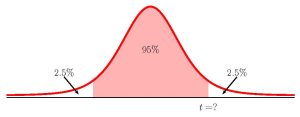
So [latex]t=1.9794...[/latex]. The 95% confidence interval is

[latex]\begin{eqnarray*} \\ \mbox{Lower Limit} & = & \overline{x}_1-\overline{x}_2-t \times \sqrt{\frac{s_1^2}{n_1}+\frac{s_2^2}{n_2}}\\ & = & 84.2-91.6-1.9794... \times \sqrt{\frac{19.4^2}{60}+\frac{18.8^2}{70}} \\ & = & -14.06  \\ \\ \mbox{Upper Limit} & = & \overline{x}_1-\overline{x}_2+t \times \sqrt{\frac{s_1^2}{n_1}+\frac{s_2^2}{n_2}}\\ & = & 84.2-91.6+1.9794... \times \sqrt{\frac{19.4^2}{60}+\frac{18.8^2}{70}} \\ & = & -0.74 \\ \\ \end{eqnarray*}[/latex]

• We are 95% confident that the difference in the mean repair time for the two photocopiers is between -14.06 minutes and -0.74 minutes.
• Because 0 is outside the confidence interval and both limits are negative, it suggests that the difference in the means [latex]\displaystyle{\mu_1-\mu_2}[/latex] is less than 0.  That is, [latex]\displaystyle{\mu_1-\mu_2 \lt 0}[/latex] ([latex]\mu_1 \lt \mu_2[/latex]).  This suggests that the mean for population 1 (photocopier A) is less than the mean for population 2 (photocopier B).  So the mean repair time for photocopier A is less than the mean repair time for photocopier B.
• When calculating the limits for the confidence interval keep all of the decimals in the [latex]t[/latex]-score and other values throughout the calculation. This will ensure that there is no round-off error in the answers. You can use Excel to do the calculation of the limits, clicking on the cells containing the [latex]t[/latex]-score and any other values, to ensure that all of the decimal places are used in the calculation.
• When writing down the interpretation of the confidence interval, make sure to include the confidence level, the actual difference in the population means captured by the confidence interval (i.e. be specific to the context of the question), and appropriate units for the limits.
• The value of the degrees of freedom must be a whole number.  After using the formula, remember to round the value down to the next whole number to get the required degrees of freedom for the [latex]t[/latex]-distribution.

Steps to Conduct a Hypothesis Test for the Difference in Two Independent Population Means with Unknown Population Standard Deviations

[latex]\begin{eqnarray*} \\ H_0: & & \mu_1-\mu_2=0 \\ \end{eqnarray*}[/latex]

[latex]\begin{eqnarray*} \\ H_a: \mu_1-\mu_2 0 & & (\mu_1 \gt \mu_2) \\ H_a: \mu_1-\mu_2 \neq 0 & & (\mu_1 \neq \mu_2) \\  \\ \end{eqnarray*}[/latex]

• Use the form of the alternative hypothesis to determine if the test is left-tailed, right-tailed, or two-tailed.
• Collect the sample information for the test and identify the significance level.

[latex]\begin{eqnarray*} t  & = &   \frac{(\overline{x}_1-\overline{x}_2)-(\mu_1-\mu_2)}{\sqrt{\frac{s_1^2}{n_1}+\frac{s_2^2}{n_2}}}  \\ \\  df  & = &   \frac{\left(\frac{s_1^2}{n_1}+\frac{s_2^2}{n_2}\right)^2}{\frac{1}{n_1-1} \times \left(\frac{s_1^2}{n_1}\right)^2+\frac{1}{n_2-1} \times \left(\frac{s_2^2}{n_2}\right)^2} \\  \\ \end{eqnarray*}[/latex]

• The results of the sample data are significant. There is sufficient evidence to conclude that the null hypothesis [latex]H_0[/latex] is an incorrect belief and that the alternative hypothesis [latex]H_a[/latex] is most likely correct.
• The results of the sample data are not significant. There is not sufficient evidence to conclude that the alternative hypothesis [latex]H_a[/latex] may be correct.
• Write down a concluding sentence specific to the context of the question.

USING EXCEL TO CALCULE THE P -VALUE FOR A HYPOTHESIS TEST ON TWO INDEPENDENT POPULATION MEANS WITH UNKNOWN POPULATION STANDARD DEVIATIONS

Assuming that the population standard deviations are unknown, the p -value for a hypothesis test on the difference in two independent population means is the area in the tail(s) of the [latex]t[/latex]-distribution.

If the p -value is the area in the left tail:

• For t-score , enter the value of [latex]t[/latex] calculated from [latex]\displaystyle{t  =  \frac{(\overline{x}_1-\overline{x}_2)-(\mu_1-\mu_2)}{\sqrt{\frac{s_1^2}{n_1}+\frac{s_2^2}{n_2}}}}[/latex].
• For the logic operator , enter true .  Note:  Because we are calculating the area under the curve, we always enter true for the logic operator.

If the p -value is the area in the right tail:

If the p -value is the sum of the area in the two tails:

• For t-score , enter the absolute value of [latex]t[/latex] calculated from [latex]\displaystyle{t  =  \frac{(\overline{x}_1-\overline{x}_2)-(\mu_1-\mu_2)}{\sqrt{\frac{s_1^2}{n_1}+\frac{s_2^2}{n_2}}}}[/latex].  Note:  In the t.dist.2t function, the value of the [latex]t[/latex]-score must be a positive number.  If the [latex]t[/latex]-score is negative, enter the absolute value of the [latex]t[/latex]-score into the t.dist.2t function.

The degrees of freedom for a [latex]t[/latex]-distribution must be a whole number .  The output from the degrees of freedom formula [latex]\displaystyle{df  =  \frac{\left(\frac{s_1^2}{n_1}+\frac{s_2^2}{n_2}\right)^2}{\frac{1}{n_1-1} \times \left(\frac{s_1^2}{n_1}\right)^2+\frac{1}{n_2-1} \times \left(\frac{s_2^2}{n_2}\right)^2}}[/latex] is almost never a whole number.  After calculating the value of [latex]df[/latex] using the formula, round the value down to the next whole number.   Remember to entered the rounded down value of [latex]df[/latex] for the degrees of freedom in the t.dist functions.

A researcher wants to study the difference between the average amount of time boys and girls aged seven to eleven spend playing sports each day. In a sample of 9 girls, the average number of hours spent playing sports per day is 2 hours with a standard deviation of 0.866 hours.  In a sample of 16 boys, the average number of hours spent playing sports per day is 3.2 hours with a standard deviation of 1 hours.  Both populations have a normal distribution.  At the 5% significance level, is there a difference in the mean amount of time boys and girls aged seven to eleven play sports each day?

Let girls be population 1 and boys be population 2.  These populations are independent because there is no relationship between the two groups.  From the questions, we have the following information:

Hypotheses:

[latex]\begin{eqnarray*} H_0: & & \mu_1-\mu_2=0 \\ H_a: & & \mu_1-\mu_2 \neq 0  \end{eqnarray*}[/latex]

This is a test on a the difference in two population means where the population standard deviation are unknown.  So we use a [latex]t[/latex]-distribution to calculate the p -value.  Because the alternative hypothesis is a [latex]\neq[/latex], the p -value is the sum of areas in the tails of the distribution.

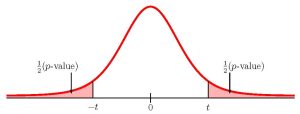
To use the t.dist.2t function, we need to calculate out the [latex]t[/latex]-score and the degrees of freedom:

[latex]\begin{eqnarray*} t & = & \frac{(\overline{x}_1-\overline{x}_2)-(\mu_1-\mu_2)}{\sqrt{\frac{s_1^2}{n_1}+\frac{s_2^2}{n_2}}} \\ & = & \frac{(2-3.2)-0}{\sqrt{\frac{0.866^2}{9}+\frac{1^2}{16}}} \\ & = & -3.1423...\\ \\ df  & = &  \frac{\left(\frac{s_1^2}{n_1}+\frac{s_2^2}{n_2}\right)^2}{\frac{1}{n_1-1} \times \left(\frac{s_1^2}{n_1}\right)^2+\frac{1}{n_2-1} \times \left(\frac{s_2^2}{n_2}\right)^2} \\    & = &  \frac{\left(\frac{0.866^2}{9}+\frac{1^2}{16}\right)^2}{\frac{1}{9-1} \times \left(\frac{0.866^2}{9}\right)^2+\frac{1}{16-1} \times \left(\frac{1^2}{16}\right)^2} \\ & = & 18.846... \\ & \Rightarrow & 18 \end{eqnarray*}[/latex]

So the p -value[latex]=0.0056[/latex].

Conclusion:

Because p -value[latex]=0.0056 \lt 0.05=\alpha[/latex], we reject the null hypothesis in favour of the alternative hypothesis.  At the 5% significance level there is enough evidence to suggest that there is a difference in the mean amount of time boys and girls aged seven to eleven play sports each day.

• The null hypothesis [latex]\mu_1-\mu_2=0[/latex] is the claim that there is no difference in the mean amount of time boys and girls spend playing sports each day.  That is, the two populations have the same mean.
• The alternative hypothesis [latex]\mu_1 -\mu_2 \neq 0[/latex] is the claim that there is a difference in the mean amount of time boys and girls spend playing sports each day ([latex]\mu_1 \neq \mu_2[/latex]).  That is, the two populations have different means.
• Keep all of the decimals throughout the calculation (i.e. in the [latex]t[/latex]-score, etc.) to avoid any round-off error in the calculation of the  p -value.  This ensures that we get the most accurate value for the  p -value.  Use Excel to do the calculations, and then click on the cells in subsequent calculations.
• The  t.dist.2t function requires that the value entered for the [latex]t[/latex]-score is positive .  A negative [latex]t[/latex]-score entered into the t.dist.2t function generates an error in Excel.  In this case, the value of the [latex]t[/latex]-score is negative, so we must enter the absolute value of this [latex]t[/latex]-score into field 1.
• The p -value of 0.0056 is a small probability compared to the significance level, and so is unlikely to happen assuming the null hypothesis is true.  This suggests that the assumption that the null hypothesis is true is most likely incorrect, and so the conclusion of the test is to reject the null hypothesis in favour of the alternative hypothesis.  In other words, there is a difference in the mean amount of time boys and girls spend playing sports each day.

A town has two colleges.  A local community group believes that students who graduate from College A have taken more math classes than the students who graduate from College B.  In a sample of 11 graduates from College A, the average is 4 math classes per graduate with a standard deviation of 1.5 math classes.  In a sample of 9 graduates from College B, the average is 3.5 math classes per graduate with a standard deviation of 1 math class.  Both populations have a normal distribution. At the 1% significance level, test the community groups claim that graduates from College A have taken more math classes than graduates from College B.

Let College A be population 1 and College B be population 2.  These populations are independent because there is no relationship between the two groups.  From the questions, we have the following information:

[latex]\begin{eqnarray*} H_0: & & \mu_1-\mu_2=0 \\ H_a: & & \mu_1-\mu_2 \gt 0  \end{eqnarray*}[/latex]

This is a test on a the difference in two population means where the population standard deviation are unknown.  So we use a [latex]t[/latex]-distribution to calculate the p -value.  Because the alternative hypothesis is a [latex]\gt[/latex], the p -value is the area in the right tail of the distribution.

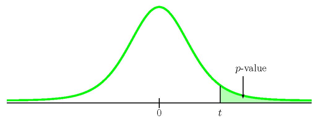
To use the t.dist.rt function, we need to calculate out the [latex]t[/latex]-score and the degrees of freedom:

[latex]\begin{eqnarray*} t & = & \frac{(\overline{x}_1-\overline{x}_2)-(\mu_1-\mu_2)}{\sqrt{\frac{s_1^2}{n_1}+\frac{s_2^2}{n_2}}} \\ & = & \frac{(4-3.5)-0}{\sqrt{\frac{1.5^2}{11}+\frac{1^2}{9}}} \\ & = & 0.8899...\\ \\  df  & = &  \frac{\left(\frac{s_1^2}{n_1}+\frac{s_2^2}{n_2}\right)^2}{\frac{1}{n_1-1} \times \left(\frac{s_1^2}{n_1}\right)^2+\frac{1}{n_2-1} \times \left(\frac{s_2^2}{n_2}\right)^2} \\    & = &  \frac{\left(\frac{1.5^2}{11}+\frac{1^2}{9}\right)^2}{\frac{1}{11-1} \times \left(\frac{1.5^2}{11}\right)^2+\frac{1}{9-1} \times \left(\frac{1^2}{9}\right)^2} \\ & = & 17.397... \\ & \Rightarrow & 17 \end{eqnarray*}[/latex]

So the p -value[latex]=0.1930[/latex].

Because p -value[latex]=0.1930 \gt 0.01=\alpha[/latex], we do not reject the null hypothesis.  At the 1% significance level there is not enough evidence to suggest that, on average, graduates of College A take more math classes than graduates of College B.

• The null hypothesis [latex]\mu_1-\mu_2=0[/latex] is the claim that the average number of math classes taken by graduates of College A equals the average number of math classes taken by graduates of College B.  That is, the two populations have the same mean.
• The alternative hypothesis [latex]\mu_1 -\mu_2 \gt 0[/latex] is the claim that, on average, graduates of College A taken more math classes than graduates of College B ([latex]\mu_1 \gt \mu_2[/latex]).
• The p -value of 0.1930 is a large probability compared to the significance level, and so is likely to happen assuming the null hypothesis is true.  This suggests that the assumption that the null hypothesis is true is most likely correct, and so the conclusion of the test is to not reject the null hypothesis.  In other words, graduates from the two colleges take, on average, the same number of math classes.

A professor at a large community college taught both an online section and a face-to-face section of his statistics course.  The professor wants to study the difference in the average score on the final exam, believing that the mean score for the online section would be lower than the face-to-face section.  The professor randomly selected 30 final exam scores from each section and recorded the scores in the tables below.

Online Section:

Face-to-Face Section:

At the 5% significance level, is the mean of the final exam score for the online section lower than the mean of the final exam score for the face-to-face section?

Let the online section be population 1 and the face-to-face section be population 2.  These populations are independent because there is no relationship between the two groups.  From the questions, we have the following information:

[latex]\begin{eqnarray*} H_0: & & \mu_1-\mu_2=0 \\ H_a: & & \mu_1-\mu_2 \lt 0  \end{eqnarray*}[/latex]

This is a test on a the difference in two population means where the population standard deviation are unknown.  So we use a [latex]t[/latex]-distribution to calculate the p -value.  Because the alternative hypothesis is a [latex]\lt[/latex], the p -value is the area in the left tail of the distribution.

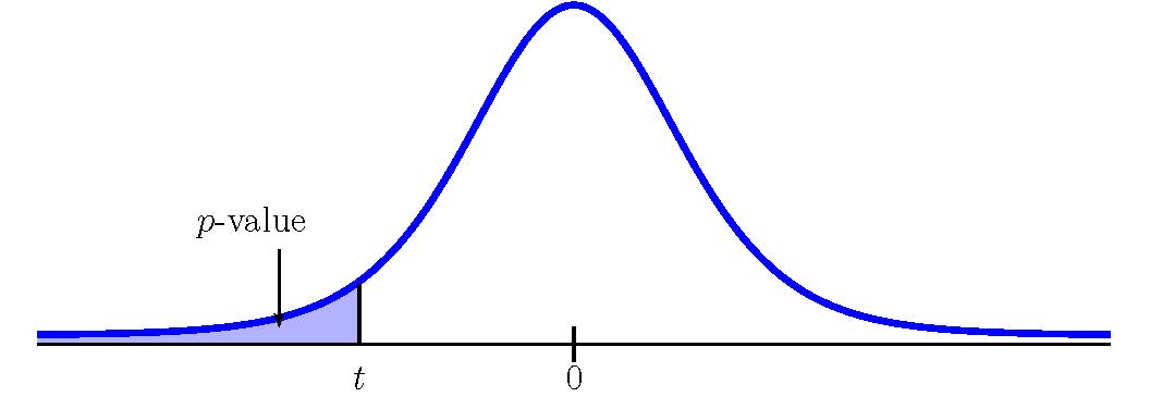
To use the t.dist  function, we need to calculate out the [latex]t[/latex]-score and the degrees of freedom:

[latex]\begin{eqnarray*} t & = & \frac{(\overline{x}_1-\overline{x}_2)-(\mu_1-\mu_2)}{\sqrt{\frac{s_1^2}{n_1}+\frac{s_2^2}{n_2}}} \\ & = & \frac{(72.85-84.98)-0}{\sqrt{\frac{16.918...^2}{30}+\frac{11.714...^2}{30}}} \\ & = & -3.228...\\ \\ df  & = &  \frac{\left(\frac{s_1^2}{n_1}+\frac{s_2^2}{n_2}\right)^2}{\frac{1}{n_1-1} \times \left(\frac{s_1^2}{n_1}\right)^2+\frac{1}{n_2-1} \times \left(\frac{s_2^2}{n_2}\right)^2} \\    & = &  \frac{\left(\frac{16.918...^2}{30}+\frac{11.714...^2}{30}\right)^2}{\frac{1}{30-1} \times \left(\frac{16.918...^2}{30}\right)^2+\frac{1}{30-1} \times \left(\frac{11.714...^2}{30}\right)^2} \\ & = & 51.608... \\ & \Rightarrow & 51 \end{eqnarray*}[/latex]

So the p -value[latex]=0.0011[/latex].

Because p -value[latex]=0.0011 \lt 0.05=\alpha[/latex], we do reject the null hypothesis in favour of the alternative hypothesis.  At the 5% significance level there is enough evidence to suggest that the mean final exam score for the online section is lower than the face-to-face section.

• The null hypothesis [latex]\mu_1-\mu_2=0[/latex] is the claim that the average final exam score is the same for both sections.  That is, the two populations have the same mean.
• The alternative hypothesis [latex]\mu_1 -\mu_2 \lt 0[/latex] is the claim that average final exam score for the online section is lower than the face-to-face section ([latex]\mu_1 \lt \mu_2[/latex]).
• Keep all of the decimals throughout the calculation (i.e. in the sample means, sample standard deviations, in the [latex]t[/latex]-score, etc.) to avoid any round-off error in the calculation of the p -value.  This ensures that we get the most accurate value for the  p -value.  Use Excel to do the calculations, and then click on the cells in subsequent calculations.
• The p -value of 0.0011 is a small probability compared to the significance level, and so is unlikely to happen assuming the null hypothesis is true.  This suggests that the assumption that the null hypothesis is true is most likely incorrect, and so the conclusion of the test is to reject the null hypothesis in favour of the alternative hypothesis.  In other words, the average final exam score for the online section is lower than for the face-to-face section.

A study is done to determine if Company A retains its workers longer than Company B. Company A samples 15 workers, and their average time with the company is 5 years with a standard deviation of 1.2 years. Company B samples 20 workers, and their average time with the company is 4.5 years with a standard deviation of 0.8 years. The populations are normally distributed.  At the 5% significance level, on average, do workers at Company A stay longer than workers at Company B?

Let Company A be population 1 and Company B be population 2.

[latex]\begin{eqnarray*} t & = & \frac{(\overline{x}_1-\overline{x}_2)-(\mu_1-\mu_2)}{\sqrt{\frac{s_1^2}{n_1}+\frac{s_2^2}{n_2}}} \\ & = & \frac{(5-4.5)-0}{\sqrt{\frac{1.2^2}{15}+\frac{0.8^2}{20}}} \\ & = & 1.3975... \\  \\ df  & = &  \frac{\left(\frac{s_1^2}{n_1}+\frac{s_2^2}{n_2}\right)^2}{\frac{1}{n_1-1} \times \left(\frac{s_1^2}{n_1}\right)^2+\frac{1}{n_2-1} \times \left(\frac{s_2^2}{n_2}\right)^2} \\    & = &  \frac{\left(\frac{1.2^2}{15}+\frac{0.8^2}{20}\right)^2}{\frac{1}{15-1} \times \left(\frac{1.2^2}{15}\right)^2+\frac{1}{20-1} \times \left(\frac{0.8^2}{20}\right)^2} \\ & = & 23.005... \\ & \Rightarrow & 23 \end{eqnarray*}[/latex]

Because p -value[latex]=0.0878 \gt 0.05=\alpha[/latex], we do not reject the null hypothesis.  At the 5% significance level there is not enough evidence to suggest that, on average, workers at Company A stay longer than workers at Company B.

Watch this video: Confidence Intervals for Two Population Means, Sigma Unknown by ExcelIsFun [16:11]

Watch this video: Hypothesis Testing for Two Population Means, Sigma Unknown by ExcelIsFun [17:29]

Concept Review

The general form of a confidence interval for the difference in two independent population means with unknown population standard deviations is

[latex]\begin{eqnarray*} \\ \mbox{Lower Limit} & = & \overline{x}_1-\overline{x}_2-t \times \sqrt{\frac{s^2_1}{n_1}+\frac{s^2_2}{n_2}} \\ \\ \mbox{Upper Limit} & = & \overline{x}_1-\overline{x}_2+t \times \sqrt{\frac{s^2_1}{n_1}+\frac{s^2_2}{n_2}} \\ \\ \end{eqnarray*}[/latex]

where [latex]t[/latex] is the positive [latex]t[/latex]-score of the [latex]t[/latex]-distribution with [latex]\displaystyle{df   =   \frac{\left(\frac{s_1^2}{n_1}+\frac{s_2^2}{n_2}\right)^2}{\frac{1}{n_1-1} \times \left(\frac{s_1^2}{n_1}\right)^2+\frac{1}{n_2-1} \times \left(\frac{s_2^2}{n_2}\right)^2}}[/latex] so that the area under the [latex]t[/latex]-distribution in between [latex]-t[/latex] and [latex]t[/latex] is [latex]C[/latex].

The hypothesis test for the difference in two independent population means with unknown population standard deviations is a well established process:

• Write down the null and alternative hypotheses in terms of the differences in the population means [latex]\mu_1-\mu_2[/latex].

[latex]\begin{eqnarray*} t & = & \frac{(\overline{x}_1-\overline{x}_2)-(\mu_1-\mu_2)}{\sqrt{\frac{s_1^2}{n_1}+\frac{s_2^2}{n_2}}} \\ \\ df &  = &  \frac{\left(\frac{s_1^2}{n_1}+\frac{s_2^2}{n_2}\right)^2}{\frac{1}{n_1-1} \times \left(\frac{s_1^2}{n_1}\right)^2+\frac{1}{n_2-1} \times \left(\frac{s_2^2}{n_2}\right)^2}\end{eqnarray*}[/latex]

• Compare the p -value to the significance level and state the outcome of the test.

Attribution

“ 10.1   Two Population Means with Unknown Standard Deviations “  and “ 10.2   Two Population Means with Known Standard Deviations “  in Introductory Statistics by OpenStax  is licensed under a  Creative Commons Attribution 4.0 International License.

Introduction to Statistics Copyright © 2022 by Valerie Watts is licensed under a Creative Commons Attribution-NonCommercial-ShareAlike 4.0 International License , except where otherwise noted.

• school Campus Bookshelves
• menu_book Bookshelves
• perm_media Learning Objects
• login Login
• how_to_reg Request Instructor Account
• hub Instructor Commons
• Download Page (PDF)
• Download Full Book (PDF)
• Periodic Table
• Physics Constants
• Scientific Calculator
• Reference & Cite
• Tools expand_more
• Readability

selected template will load here

This action is not available.

8.6: Hypothesis Test of a Single Population Mean with Examples

• Last updated
• Save as PDF
• Page ID 130297

Steps for performing Hypothesis Test of a Single Population Mean

Step 1: State your hypotheses about the population mean. Step 2: Summarize the data. State a significance level. State and check conditions required for the procedure

• Find or identify the sample size, n, the sample mean, \(\bar{x}\) and the sample standard deviation, s .

The sampling distribution for the one-mean test statistic is, approximately, T- distribution if the following conditions are met

• Sample is random with independent observations .
• Sample is large. The population must be Normal or the sample size must be at least 30.

Step 3: Perform the procedure based on the assumption that \(H_{0}\) is true

• Find the Estimated Standard Error: \(SE=\frac{s}{\sqrt{n}}\).
• Compute the observed value of the test statistic: \(T_{obs}=\frac{\bar{x}-\mu_{0}}{SE}\).
• Check the type of the test (right-, left-, or two-tailed)
• Find the p-value in order to measure your level of surprise.

Step 4: Make a decision about \(H_{0}\) and \(H_{a}\)

• Do you reject or not reject your null hypothesis?

Step 5: Make a conclusion

• What does this mean in the context of the data?

The following examples illustrate a left-, right-, and two-tailed test.

Example \(\pageindex{1}\).

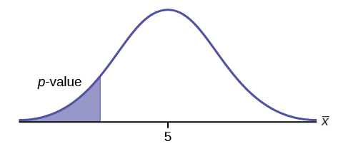
\(H_{0}: \mu = 5, H_{a}: \mu < 5\)

Test of a single population mean. \(H_{a}\) tells you the test is left-tailed. The picture of the \(p\)-value is as follows:

Exercise \(\PageIndex{1}\)

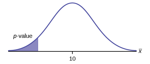
\(H_{0}: \mu = 10, H_{a}: \mu < 10\)

Assume the \(p\)-value is 0.0935. What type of test is this? Draw the picture of the \(p\)-value.

left-tailed test

Example \(\PageIndex{2}\)

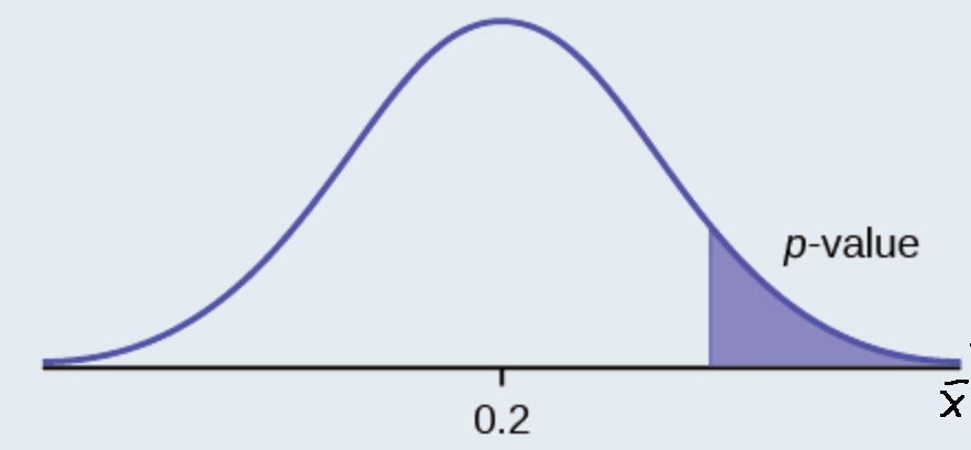
\(H_{0}: \mu \leq 0.2, H_{a}: \mu > 0.2\)

This is a test of a single population proportion. \(H_{a}\) tells you the test is right-tailed . The picture of the p -value is as follows:

Exercise \(\PageIndex{2}\)

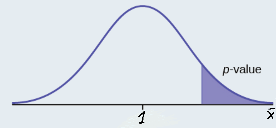
\(H_{0}: \mu \leq 1, H_{a}: \mu > 1\)

Assume the \(p\)-value is 0.1243. What type of test is this? Draw the picture of the \(p\)-value.

right-tailed test

Example \(\PageIndex{3}\)

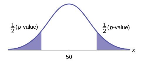
\(H_{0}: \mu = 50, H_{a}: \mu \neq 50\)

This is a test of a single population mean. \(H_{a}\) tells you the test is two-tailed . The picture of the \(p\)-value is as follows.

Exercise \(\PageIndex{3}\)

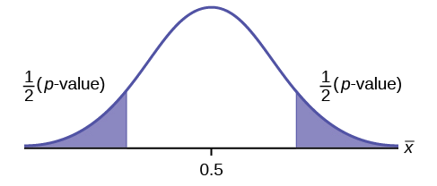
\(H_{0}: \mu = 0.5, H_{a}: \mu \neq 0.5\)

Assume the p -value is 0.2564. What type of test is this? Draw the picture of the \(p\)-value.

two-tailed test

Full Hypothesis Test Examples

Example \(\pageindex{4}\).

Statistics students believe that the mean score on the first statistics test is 65. A statistics instructor thinks the mean score is higher than 65. He samples ten statistics students and obtains the scores 65 65 70 67 66 63 63 68 72 71. He performs a hypothesis test using a 5% level of significance. The data are assumed to be from a normal distribution.

Set up the hypothesis test:

A 5% level of significance means that \(\alpha = 0.05\). This is a test of a single population mean .

\(H_{0}: \mu = 65  H_{a}: \mu > 65\)

Since the instructor thinks the average score is higher, use a "\(>\)". The "\(>\)" means the test is right-tailed.

Determine the distribution needed:

Random variable: \(\bar{X} =\) average score on the first statistics test.

Distribution for the test: If you read the problem carefully, you will notice that there is no population standard deviation given . You are only given \(n = 10\) sample data values. Notice also that the data come from a normal distribution. This means that the distribution for the test is a student's \(t\).

Use \(t_{df}\). Therefore, the distribution for the test is \(t_{9}\) where \(n = 10\) and \(df = 10 - 1 = 9\).

The sample mean and sample standard deviation are calculated as 67 and 3.1972 from the data.

Calculate the \(p\)-value using the Student's \(t\)-distribution:

\[t_{obs} = \dfrac{\bar{x}-\mu_{\bar{x}}}{\left(\dfrac{s}{\sqrt{n}}\right)}=\dfrac{67-65}{\left(\dfrac{3.1972}{\sqrt{10}}\right)}\]

Use the T-table or Excel's t_dist() function to find p-value:

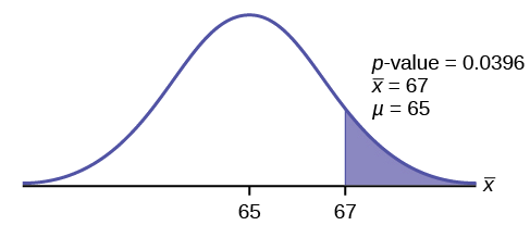
\(p\text{-value} = P(\bar{x} > 67) =P(T >1.9782 )= 1-0.9604=0.0396\)

Interpretation of the p -value: If the null hypothesis is true, then there is a 0.0396 probability (3.96%) that the sample mean is 65 or more.

Compare \(\alpha\) and the \(p-\text{value}\):

Since \(α = 0.05\) and \(p\text{-value} = 0.0396\). \(\alpha > p\text{-value}\).

Make a decision: Since \(\alpha > p\text{-value}\), reject \(H_{0}\).

This means you reject \(\mu = 65\). In other words, you believe the average test score is more than 65.

Conclusion: At a 5% level of significance, the sample data show sufficient evidence that the mean (average) test score is more than 65, just as the math instructor thinks.

The \(p\text{-value}\) can easily be calculated.

Put the data into a list. Press STAT and arrow over to TESTS . Press 2:T-Test . Arrow over to Data and press ENTER . Arrow down and enter 65 for \(\mu_{0}\), the name of the list where you put the data, and 1 for Freq: . Arrow down to \(\mu\): and arrow over to \(> \mu_{0}\). Press ENTER . Arrow down to Calculate and press ENTER . The calculator not only calculates the \(p\text{-value}\) (p = 0.0396) but it also calculates the test statistic ( t -score) for the sample mean, the sample mean, and the sample standard deviation. \(\mu > 65\) is the alternative hypothesis. Do this set of instructions again except arrow to Draw (instead of Calculate ). Press ENTER . A shaded graph appears with \(t = 1.9781\) (test statistic) and \(p = 0.0396\) (\(p\text{-value}\)). Make sure when you use Draw that no other equations are highlighted in \(Y =\) and the plots are turned off.

Exercise \(\PageIndex{4}\)

It is believed that a stock price for a particular company will grow at a rate of $5 per week with a standard deviation of $1. An investor believes the stock won’t grow as quickly. The changes in stock price is recorded for ten weeks and are as follows: $4, $3, $2, $3, $1, $7, $2, $1, $1, $2. Perform a hypothesis test using a 5% level of significance. State the null and alternative hypotheses, find the p -value, state your conclusion, and identify the Type I and Type II errors.

• \(H_{0}: \mu = 5\)
• \(H_{a}: \mu < 5\)
• \(p = 0.0082\)

Because \(p < \alpha\), we reject the null hypothesis. There is sufficient evidence to suggest that the stock price of the company grows at a rate less than $5 a week.

• Type I Error: To conclude that the stock price is growing slower than $5 a week when, in fact, the stock price is growing at $5 a week (reject the null hypothesis when the null hypothesis is true).
• Type II Error: To conclude that the stock price is growing at a rate of $5 a week when, in fact, the stock price is growing slower than $5 a week (do not reject the null hypothesis when the null hypothesis is false).

Example \(\PageIndex{5}\)

The National Institute of Standards and Technology provides exact data on conductivity properties of materials. Following are conductivity measurements for 11 randomly selected pieces of a particular type of glass.

1.11; 1.07; 1.11; 1.07; 1.12; 1.08; .98; .98 1.02; .95; .95

Is there convincing evidence that the average conductivity of this type of glass is greater than one? Use a significance level of 0.05. Assume the population is normal.

Let’s follow a four-step process to answer this statistical question.

• \(H_{0}: \mu \leq 1\)
• \(H_{a}: \mu > 1\)
• Plan : We are testing a sample mean without a known population standard deviation. Therefore, we need to use a Student's-t distribution. Assume the underlying population is normal.
• Do the calculations : \(p\text{-value} ( = 0.036)\)

4. State the Conclusions : Since the \(p\text{-value} (= 0.036)\) is less than our alpha value, we will reject the null hypothesis. It is reasonable to state that the data supports the claim that the average conductivity level is greater than one.

The hypothesis test itself has an established process. This can be summarized as follows:

• Determine \(H_{0}\) and \(H_{a}\). Remember, they are contradictory.
• Determine the random variable.
• Determine the distribution for the test.
• Draw a graph, calculate the test statistic, and use the test statistic to calculate the \(p\text{-value}\). (A t -score is an example of test statistics.)
• Compare the preconceived α with the p -value, make a decision (reject or do not reject H 0 ), and write a clear conclusion using English sentences.

Notice that in performing the hypothesis test, you use \(\alpha\) and not \(\beta\). \(\beta\) is needed to help determine the sample size of the data that is used in calculating the \(p\text{-value}\). Remember that the quantity \(1 – \beta\) is called the Power of the Test . A high power is desirable. If the power is too low, statisticians typically increase the sample size while keeping α the same.If the power is low, the null hypothesis might not be rejected when it should be.

• Data from Amit Schitai. Director of Instructional Technology and Distance Learning. LBCC.
• Data from Bloomberg Businessweek . Available online at www.businessweek.com/news/2011- 09-15/nyc-smoking-rate-falls-to-record-low-of-14-bloomberg-says.html.
• Data from energy.gov. Available online at http://energy.gov (accessed June 27. 2013).
• Data from Gallup®. Available online at www.gallup.com (accessed June 27, 2013).
• Data from Growing by Degrees by Allen and Seaman.
• Data from La Leche League International. Available online at www.lalecheleague.org/Law/BAFeb01.html.
• Data from the American Automobile Association. Available online at www.aaa.com (accessed June 27, 2013).
• Data from the American Library Association. Available online at www.ala.org (accessed June 27, 2013).
• Data from the Bureau of Labor Statistics. Available online at http://www.bls.gov/oes/current/oes291111.htm .
• Data from the Centers for Disease Control and Prevention. Available online at www.cdc.gov (accessed June 27, 2013)
• Data from the U.S. Census Bureau, available online at quickfacts.census.gov/qfd/states/00000.html (accessed June 27, 2013).
• Data from the United States Census Bureau. Available online at www.census.gov/hhes/socdemo/language/.
• Data from Toastmasters International. Available online at http://toastmasters.org/artisan/deta...eID=429&Page=1 .
• Data from Weather Underground. Available online at www.wunderground.com (accessed June 27, 2013).
• Federal Bureau of Investigations. “Uniform Crime Reports and Index of Crime in Daviess in the State of Kentucky enforced by Daviess County from 1985 to 2005.” Available online at http://www.disastercenter.com/kentucky/crime/3868.htm (accessed June 27, 2013).
• “Foothill-De Anza Community College District.” De Anza College, Winter 2006. Available online at research.fhda.edu/factbook/DA...t_da_2006w.pdf.
• Johansen, C., J. Boice, Jr., J. McLaughlin, J. Olsen. “Cellular Telephones and Cancer—a Nationwide Cohort Study in Denmark.” Institute of Cancer Epidemiology and the Danish Cancer Society, 93(3):203-7. Available online at http://www.ncbi.nlm.nih.gov/pubmed/11158188 (accessed June 27, 2013).
• Rape, Abuse & Incest National Network. “How often does sexual assault occur?” RAINN, 2009. Available online at www.rainn.org/get-information...sexual-assault (accessed June 27, 2013).

T-test for two Means – Unknown Population Standard Deviations

Instructions : Use this T-Test Calculator for two Independent Means calculator to conduct a t-test for two population means (\(\mu_1\) and \(\mu_2\)), with unknown population standard deviations. This test apply when you have two-independent samples, and the population standard deviations \(\sigma_1\) and \(\sigma_2\) and not known. Please select the null and alternative hypotheses, type the significance level, the sample means, the sample standard deviations, the sample sizes, and the results of the t-test for two independent samples will be displayed for you:

The T-test for Two Independent Samples

More about the t-test for two means so you can better interpret the output presented above: A t-test for two means with unknown population variances and two independent samples is a hypothesis test that attempts to make a claim about the population means (\(\mu_1\) and \(\mu_2\)).

More specifically, a t-test uses sample information to assess how plausible it is for the population means \(\mu_1\) and \(\mu_2\) to be equal. The test has two non-overlapping hypotheses, the null and the alternative hypothesis.

The null hypothesis is a statement about the population means, specifically the assumption of no effect, and the alternative hypothesis is the complementary hypothesis to the null hypothesis.

Properties of the two sample t-test

The main properties of a two sample t-test for two population means are:

• Depending on our knowledge about the "no effect" situation, the t-test can be two-tailed, left-tailed or right-tailed
• The main principle of hypothesis testing is that the null hypothesis is rejected if the test statistic obtained is sufficiently unlikely under the assumption that the null hypothesis is true
• The p-value is the probability of obtaining sample results as extreme or more extreme than the sample results obtained, under the assumption that the null hypothesis is true
• In a hypothesis tests there are two types of errors. Type I error occurs when we reject a true null hypothesis, and the Type II error occurs when we fail to reject a false null hypothesis

How do you compute the t-statistic for the t test for two independent samples?

The formula for a t-statistic for two population means (with two independent samples), with unknown population variances shows us how to calculate t-test with mean and standard deviation and it depends on whether the population variances are assumed to be equal or not. If the population variances are assumed to be unequal, then the formula is:

On the other hand, if the population variances are assumed to be equal, then the formula is:

Normally, the way of knowing whether the population variances must be assumed to be equal or unequal is by using an F-test for equality of variances.

With the above t-statistic, we can compute the corresponding p-value, which allows us to assess whether or not there is a statistically significant difference between two means.

Why is it called t-test for independent samples?

This is because the samples are not related with each other, in a way that the outcomes from one sample are unrelated from the other sample. If the samples are related (for example, you are comparing the answers of husbands and wives, or identical twins), you should use a t-test for paired samples instead .

What if the population standard deviations are known?

The main purpose of this calculator is for comparing two population mean when sigma is unknown for both populations. In case that the population standard deviations are known, then you should use instead this z-test for two means .

Related Calculators

log in to your account

Reset password.

• school Campus Bookshelves
• menu_book Bookshelves
• perm_media Learning Objects
• login Login
• how_to_reg Request Instructor Account
• hub Instructor Commons
• Download Page (PDF)
• Download Full Book (PDF)
• Periodic Table
• Physics Constants
• Scientific Calculator
• Reference & Cite
• Tools expand_more
• Readability

selected template will load here

This action is not available.

3.5: Hypothesis Test about a Variance

• Last updated
• Save as PDF
• Page ID 2887

• Diane Kiernan
• SUNY College of Environmental Science and Forestry via OpenSUNY

Hypothesis Test about a Variance

When people think of statistical inference, they usually think of inferences involving population means or proportions. However, the particular population parameter needed to answer an experimenter’s practical questions varies from one situation to another, and sometimes a population’s variability is more important than its mean. Thus, product quality is often defined in terms of low variability.

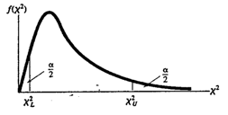
Sample variance \(s^2\) can be used for inferences concerning a population variance \(\sigma^2\) . For a random sample of n measurements drawn from a normal population with mean μ and variance \(\sigma^2\) , the value \(s^2\) provides a point estimate for \(\sigma^2\) . In addition, the quantity \(\frac {(n-1)s^2}{\sigma^2}\) follows a Chi-square (\(\chi^{2}\)) distribution, with \(df = n – 1\).

The properties of Chi-square ( \(\chi^{2}\) ) distribution are:

• Unlike Z and t distributions, the values in a chi-square distribution are all positive.
• The chi-square distribution is asymmetric, unlike the Z and t distributions.
• There are many chi-square distributions. We obtain a particular one by specifying the degrees of freedom \((df = n – 1)\) associated with the sample variances \(s^2\) .

One-sample (\(\chi^{2}\) ) test for testing the hypotheses:

Null hypothesis: \(H_0: \sigma^{2} = \sigma^{2}_{0}\)(constant)

Alternative hypothesis:

• \(H_a: σ^2 > \sigma_{0}^{2}\)(one-tailed), reject \(H_0\) if the observed \(\chi^2 > \chi_{U}^{2}\)(upper-tail value at α).
• \(H_a: σ^2 <\sigma_{0}^{2}\) (one-tailed), reject \(H_0\) if the observed \(\chi^2 < \chi_{L}^{2}\)(lower-tail value at α).
• \(H_a: σ^2 ≠ \sigma_{0}^{2}\) (two-tailed), reject \(H_0\) if the observed \(\chi^2 > \chi_{U}^{2}\)or \(\chi^{2} < \chi_{L}^{2}\)at α/2.

where the \(\chi^2\) critical value in the rejection region is based on degrees of freedom \(df = n – 1\) and a specified significance level of α .

Test statistic: \[\chi^2 = \frac{(n-1)S^2}{\sigma _{0}^{2}}\]

As with previous sections, if the test statistic falls in the rejection zone set by the critical value, you will reject the null hypothesis.

Example \(\PageIndex{1}\):

A forester wants to control a dense understory of striped maple that is interfering with desirable hardwood regeneration using a mist blower to apply an herbicide treatment. She wants to make sure that treatment has a consistent application rate, in other words, low variability not exceeding 0.25 gal./acre (0.06 gal.2). She collects sample data (n = 11) on this type of mist blower and gets a sample variance of 0.064 gal.2 Using a 5% level of significance, test the claim that the variance is significantly greater than 0.06 gal.2

\(H_0: \sigma^{2} = 0.06\)

\(H_1: \sigma^{2} >0.06\)

The critical value is 18.307. Any test statistic greater than this value will cause you to reject the null hypothesis.

The test statistic is

\[\chi^2 = \frac {(n-1)S^2}{\sigma_{0}^{2}}=\frac {(11-1)0.064}{0.06}=10.667 \nonumber \]

We fail to reject the null hypothesis. The forester does NOT have enough evidence to support the claim that the variance is greater than 0.06 gal.2 You can also estimate the p-value using the same method as for the student t-table. Go across the row for degrees of freedom until you find the two values that your test statistic falls between. In this case going across the row 10, the two table values are 4.865 and 15.987. Now go up those two columns to the top row to estimate the p-value (0.1-0.9). The p-value is greater than 0.1 and less than 0.9. Both are greater than the level of significance (0.05) causing us to fail to reject the null hypothesis.

Software Solutions

(referring to Ex. \(\PageIndex{1}\) )

Test and CI for One Variance

The chi-square method is only for the normal distribution.

Excel does not offer 1-sample \(\chi^2\) testing.