travel assignment

• Travel Jobs
• Licensure Guide
• Exclusive Jobs

Let's Get Started

• Setting Up Your Stability Account
• National Travel Assignments
• The Best Paying Travel Nursing Specialties
• The Best Paying Travel Allied Specialties

Prepare for Your Assignment

• Housing Guides
• Maintaining Work Life Balance
• Stability Stories
• Contract Registered Nursing
• Contract Registered Nursing 101
• Nursing Certifications
• International Contract Registered Nursing Guide
• Nursing FAQs
• Working with a Travel Nurse Agency
• Nursing Compact States
• Contract Allied
• Your Guide To Allied Health Travel Jobs
• Our Company

Take charge of your healthcare career

566+ Reviews

61+ Reviews

40+ Reviews

73+ Reviews

Stability for Healthcare Professionals

You deserve a job that fits around your life and goals– not the other way around. Our self-service job board and attentive team are here to secure that ideal opportunity.

Stability for Managed Services Partner

We take the hassle off your desk and ensure you always have your staffing needs met by our nationwide network of healthcare professionals.

Market-Leading Pay Rates And Nationwide Opportunities

Connect with top-rated hospitals, see pay details, benefits, and hospital information upfront, same day pay available.

Assignment Options

Our job search is built with your schedule in mind, open 24/7, 365 days a year for you to explore.

• Travel and Local Positions
• Assignments updated hourly
• Permanent Staffing
• Exclusive Opportunities

Stability Experience

Our recruiters are here to assign you every stay of the way…

We also provide you with:

• Career counseling
• 24/7 Job Search
• Paid Time Off
• 401k Matching

How Stability Works

Search for jobs based on your preference, match with the perfect job for you, and fast track to interview, start assignment, start assignment.

Specialty Jobs

• Tele-Med Surg

Highest-Paying Locations

Highest Paying

$2563 /Week

$3064 /Week

$5948 /Week

$2426 /Week

$4244 /Week

$2798 /Week

Want To See More?

Start building your career today.

Earned the Joint Commission Gold Seal of Approval.

Explore Jobs

• Salary Guide
• Career Building
• Life & Environment
• DAISY Award
• Managed Services Partner
• Careers – Clinician
• Careers – Corporate
• [email protected]
• 855-742-4767
• Cookie Policy
• Privacy Policy
• Terms & Conditions

• Search Jobs
• Get Started

Featured Jobs

Already have a Host Healthcare profile? Log In to view all job details

New to travel healthcare? Sign up  to get started with one of our specialized recruiters.

• RN 13 Weeks Days Estimated Total Pay $4,563.08 - $4,753.06 /wk*

*Includes estimated wage of $63.88 - $70.88/hr and non-taxable benefits if eligible

• Vascular/ECHO Technologist 14 Weeks Days Estimated Total Pay $4,030.46 - $4,220.44 /wk*

*Includes estimated wage of $65.79 - $72.79/hr and non-taxable benefits if eligible

• RN 13 Weeks Days Estimated Total Pay $3,856.69 - $4,046.67 /wk*

*Includes estimated wage of $49.19 - $56.19/hr and non-taxable benefits if eligible

• RN 13 Weeks Days Estimated Total Pay $3,837.32 - $4,027.30 /wk*

*Includes estimated wage of $71.62 - $78.62/hr and non-taxable benefits if eligible

• RN 13 Weeks Days Estimated Total Pay $3,721.69 - $3,911.67 /wk*

*Includes estimated wage of $58.24 - $65.24/hr and non-taxable benefits if eligible

*Includes estimated wage of $47.39 - $54.39/hr and non-taxable benefits if eligible

• RN 13 Weeks Days Estimated Total Pay $3,588.46 - $3,778.44 /wk*

*Includes estimated wage of $53.69 - $60.69/hr and non-taxable benefits if eligible

• CT Technologist 13 Weeks Days Estimated Total Pay $3,386.53 - $3,576.51 /wk*

*Includes estimated wage of $21.34 - $28.34/hr and non-taxable benefits if eligible

• Cath Lab Tech 13 Weeks Variable Estimated Total Pay $3,363.52 - $3,553.50 /wk*

*Includes estimated wage of $36.69 - $43.69/hr and non-taxable benefits if eligible

• Physical Therapist 13 Weeks Days Estimated Total Pay $3,338.24 - $3,528.22 /wk*

*Includes estimated wage of $31.51 - $38.51/hr and non-taxable benefits if eligible

• Radiation Therapist 13 Weeks Days Estimated Total Pay $3,324.35 - $3,514.33 /wk*

*Includes estimated wage of $43.41 - $50.41/hr and non-taxable benefits if eligible

• RN 13 Weeks Days Estimated Total Pay $3,321.52 - $3,511.50 /wk*

*Includes estimated wage of $39.49 - $46.49/hr and non-taxable benefits if eligible

• RN 13 Weeks Days, Variable Estimated Total Pay $3,321.52 - $3,511.50 /wk*

*Includes estimated wage of $28.99 - $35.99/hr and non-taxable benefits if eligible

• RN 26 Weeks Days Estimated Total Pay $3,297.21 - $3,476.00 /wk*

• RN 13 Weeks Days Estimated Total Pay $3,203.08 - $3,393.06 /wk*

*Includes estimated wage of $28.13 - $35.13/hr and non-taxable benefits if eligible

Find Travel Healthcare Jobs

Travel healthcare offers healthcare professionals new career opportunities that involve travel, growth, and excitement. At Host Healthcare, we are dedicated to providing travel nurses, travel therapists, and travel allied professionals with the assignment of their dreams. We have travel healthcare jobs in all 50 states and believe in matching healthcare professionals with travel assignments that fit their career, lifestyle, and travel goals. Our travel healthcare job listings provide high-paying assignment salaries and allow healthcare professionals to gain experience while traveling to any destination across the United States. Whether you’re an allied health professional or registered nurse looking for a travel assignment in New York or Alaska, you’re certain to find the perfect travel healthcare job.

Sign up to get started with one of our dedicated and friendly recruiters or use the search to find your perfect travel assignment.

You'll Love Our Recruiters

Here’s what our travelers have to say about working with us

TRAVELER REVIEWS MEET OUR TEAM

Recognized by

The #1 .cls-1{fill:#9ce7a7;stroke-width:0px;} Rated Travel Nursing Agency

Check out these reviews from real host healthcare travelers..

Host Healthcare is amazing! Best travel co out there! Amanda is the recruiter I have & she is wonderful. She is there from the beginning. From searching for the perfect assignment throughout completion of a contract - Amanda is there for me! Host Healthcare treats their nurses so well

Amanda Goad is the most amazing recruiter I have worked with. She is the most responsive and go-getter. She is in constant contact with you or hospitals to get you offers and/or advocating for you. She is super motivated and helpful. If you have the opportunity to use her, you will not regret it.

Needed to move across country to be next to my partner, but blindly jumping into a full time job for a hospital system I was not familiar with was out of the question. Host Healthcare (Natalie G specifically) stood by me and helped me fulfill my absurdly specific requests. I was a first time time traveler and I couldn't have made it without the support I received!

Just finished my first contract with Host Healthcare (fifth overall) and they were amazing! Specifically my recruiter Jenny Berroth. Jenny was so helpful and easy to communicate with. I had a couple issues come up and Jenny was all over them and took care of everything so I could just concentrate on being a nurse, while she handled the rest. I can’t recommend Host and Jenny enough! You have to give Host and Jenny a try, you’ll be glad you did!

Start Your Journey Today

Got questions we’ve got answers..

Chat Email Give Us A Call

(712) 336-0800

Travel Nurse Jobs & Travel Nursing Assistant Jobs

If you're interested in working and venturing away from home, travel assignments are perfect for you travel and explore what the world has to offer, all while doing what you do best — providing quality care., travel contract jobs for nurses & nursing assistants.

Your opportunities with GrapeTree are endless! Along with per-diem shifts and local long-term assignments, our healthcare professionals have the opportunity to travel and explore new areas without giving up a regular income. Travel contracts are 8-13 weeks in length, offer opportunities to work outside a 50 mile radius of your home, and include travel + housing stipends. Mesh your career with new personal life experiences by becoming a travel CNA/STNA, LPN, or RN with GrapeTree!

You get the best of both worlds. Earn a competitive wage while exploring your surroundings in your down time.

Live in, make memories in, and explore a new area with every new travel assignment

Receive a weekly, non-taxed per diem, to assist with travel, meals, housing, incidentals, and other necessary expenses.

Guaranteed hours

Your schedule is set from the moment you are booked into a travel assignment with GrapeTree.

We currently offer travel opportunities throughout the states below – but we are still expanding! Check out all of the fun things to do in each of our states and pick your next home-away-from-home.

Make More With Travel Contracts

The weekly package range for travel assignments is a combination of hourly taxed rate and a weekly non-taxed per diem reimbursement to cover housing, meals, incidentals, and other necessary costs. Package amount is based on facility type, specialty, location, and certification of healthcare professional.

CN A s /STN A s

$1,200-$1,700 per week.

Must have 6 months of experience working as a CNA or STNA.

$1,600-$2,000 PER WEEK

Must have 1 year of experience working as an LPN.

$2,000-$2,700

Must have 1 year of experience working as an RN.

Your h ome address must be least 50 miles away from the facility to qualify for travel pay rates. Contracts are available as local assignments at a lower pay rate for those whose home address is less than 50 miles away from the facility address.

Get Certified in Other States

Only certified to work in your home state? No problem! While each state has their own process for becoming licensed, it is easy to get your license transferred. This process is called getting "reciprocity" or "endorsement." Our team has compiled a list of all our states' registries so that you can easily transfer your license. Give our team a call to learn more about getting reimbursed for gaining reciprocity in other states! Click the button below to get started.

The Perks of Travel A ssignments

Flexibility.

You have the flexibility to choose where you go and what assignments you take on.

Avoid Burnout

Experience higher job satisfaction working in a travel assignment by avoiding overtime.

Gain Knowledge

Explore what you love about nursing by working with more people in diverse settings.

Career Advancement

Strengthen your experience an build up your resume to show that you thrive in all environments.

What People Are Saying

I've been working and traveling with GrapeTree Medical Staffing for about five months now and have loved every minute of it! The communication is great, the pay is excellent and I love how flexible they are! If you are looking for a great company to work for I highly recommend GrapeTree!

Alissa | Travel CNA

Got questions we've got answers..

Book Your Dream A ssignment

Our team is waiting to hear from you! Learn more about our travel opportunities or book your dream assignment by giving us a call at (712) 336-0800 and select option 4.

Interested in More Information?

• Articles   >

The Moscow Metro Museum of Art: 10 Must-See Stations

There are few times one can claim having been on the subway all afternoon and loving it, but the Moscow Metro provides just that opportunity.  While many cities boast famous public transport systems—New York’s subway, London’s underground, San Salvador’s chicken buses—few warrant hours of exploration.  Moscow is different: Take one ride on the Metro, and you’ll find out that this network of railways can be so much more than point A to B drudgery.

The Metro began operating in 1935 with just thirteen stations, covering less than seven miles, but it has since grown into the world’s third busiest transit system ( Tokyo is first ), spanning about 200 miles and offering over 180 stops along the way.  The construction of the Metro began under Joseph Stalin’s command, and being one of the USSR’s most ambitious building projects, the iron-fisted leader instructed designers to create a place full of svet (radiance) and svetloe budushchee (a radiant future), a palace for the people and a tribute to the Mother nation.

Consequently, the Metro is among the most memorable attractions in Moscow.  The stations provide a unique collection of public art, comparable to anything the city’s galleries have to offer and providing a sense of the Soviet era, which is absent from the State National History Museum.  Even better, touring the Metro delivers palpable, experiential moments, which many of us don’t get standing in front of painting or a case of coins.

Though tours are available , discovering the Moscow Metro on your own provides a much more comprehensive, truer experience, something much less sterile than following a guide.  What better place is there to see the “real” Moscow than on mass transit: A few hours will expose you to characters and caricatures you’ll be hard-pressed to find dining near the Bolshoi Theater.  You become part of the attraction, hear it in the screech of the train, feel it as hurried commuters brush by: The Metro sucks you beneath the city and churns you into the mix.

With the recommendations of our born-and-bred Muscovite students, my wife Emma and I have just taken a self-guided tour of what some locals consider the top ten stations of the Moscow Metro. What most satisfied me about our Metro tour was the sense of adventure .  I loved following our route on the maps of the wagon walls as we circled the city, plotting out the course to the subsequent stops; having the weird sensation of being underground for nearly four hours; and discovering the next cavern of treasures, playing Indiana Jones for the afternoon, piecing together fragments of Russia’s mysterious history.  It’s the ultimate interactive museum.

Top Ten Stations (In order of appearance)

Kievskaya station.

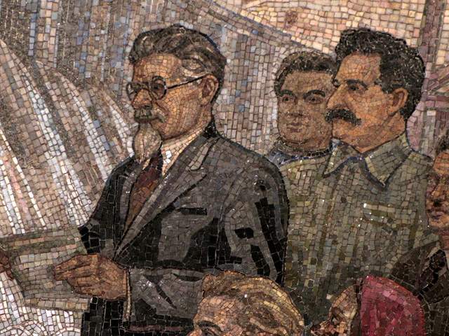
Kievskaya Station went public in March of 1937, the rails between it and Park Kultury Station being the first to cross the Moscow River.  Kievskaya is full of mosaics depicting aristocratic scenes of Russian life, with great cameo appearances by Lenin, Trotsky, and Stalin.  Each work has a Cyrillic title/explanation etched in the marble beneath it; however, if your Russian is rusty, you can just appreciate seeing familiar revolutionary dates like 1905 ( the Russian Revolution ) and 1917 ( the October Revolution ).

Mayakovskaya Station

Mayakovskaya Station ranks in my top three most notable Metro stations. Mayakovskaya just feels right, done Art Deco but no sense of gaudiness or pretention.  The arches are adorned with rounded chrome piping and create feeling of being in a jukebox, but the roof’s expansive mosaics of the sky are the real showstopper.  Subjects cleverly range from looking up at a high jumper, workers atop a building, spires of Orthodox cathedrals, to nimble aircraft humming by, a fleet of prop planes spelling out CCCP in the bluest of skies.

Novoslobodskaya Station

Novoslobodskaya is the Metro’s unique stained glass station.  Each column has its own distinctive panels of colorful glass, most of them with a floral theme, some of them capturing the odd sailor, musician, artist, gardener, or stenographer in action.  The glass is framed in Art Deco metalwork, and there is the lovely aspect of discovering panels in the less frequented haunches of the hall (on the trackside, between the incoming staircases).  Novosblod is, I’ve been told, the favorite amongst out-of-town visitors.

Komsomolskaya Station

Komsomolskaya Station is one of palatial grandeur.  It seems both magnificent and obligatory, like the presidential palace of a colonial city.  The yellow ceiling has leafy, white concrete garland and a series of golden military mosaics accenting the tile mosaics of glorified Russian life.  Switching lines here, the hallway has an Alice-in-Wonderland feel, impossibly long with decorative tile walls, culminating in a very old station left in a remarkable state of disrepair, offering a really tangible glimpse behind the palace walls.

Dostoevskaya Station

Dostoevskaya is a tribute to the late, great hero of Russian literature .  The station at first glance seems bare and unimpressive, a stark marble platform without a whiff of reassembled chips of tile.  However, two columns have eerie stone inlay collages of scenes from Dostoevsky’s work, including The Idiot , The Brothers Karamazov , and Crime and Punishment.   Then, standing at the center of the platform, the marble creates a kaleidoscope of reflections.  At the entrance, there is a large, inlay portrait of the author.

Chkalovskaya Station

Chkalovskaya does space Art Deco style (yet again).  Chrome borders all.  Passageways with curvy overhangs create the illusion of walking through the belly of a chic, new-age spacecraft.  There are two (kos)mosaics, one at each end, with planetary subjects.  Transferring here brings you above ground, where some rather elaborate metalwork is on display.  By name similarity only, I’d expected Komsolskaya Station to deliver some kosmonaut décor; instead, it was Chkalovskaya that took us up to the space station.

Elektrozavodskaya Station

Elektrozavodskaya is full of marble reliefs of workers, men and women, laboring through the different stages of industry.  The superhuman figures are round with muscles, Hollywood fit, and seemingly undeterred by each Herculean task they respectively perform.  The station is chocked with brass, from hammer and sickle light fixtures to beautiful, angular framework up the innards of the columns.  The station’s art pieces are less clever or extravagant than others, but identifying the different stages of industry is entertaining.

Baumanskaya Statio

Baumanskaya Station is the only stop that wasn’t suggested by the students.  Pulling in, the network of statues was just too enticing: Out of half-circle depressions in the platform’s columns, the USSR’s proud and powerful labor force again flaunts its success.  Pilots, blacksmiths, politicians, and artists have all congregated, posing amongst more Art Deco framing.  At the far end, a massive Soviet flag dons the face of Lenin and banners for ’05, ’17, and ‘45.  Standing in front of the flag, you can play with the echoing roof.

Ploshchad Revolutsii Station

Novokuznetskaya Station

Novokuznetskaya Station finishes off this tour, more or less, where it started: beautiful mosaics.  This station recalls the skyward-facing pieces from Mayakovskaya (Station #2), only with a little larger pictures in a more cramped, very trafficked area.  Due to a line of street lamps in the center of the platform, it has the atmosphere of a bustling market.  The more inventive sky scenes include a man on a ladder, women picking fruit, and a tank-dozer being craned in.  The station’s also has a handsome black-and-white stone mural.

Here is a map and a brief description of our route:

Start at (1)Kievskaya on the “ring line” (look for the squares at the bottom of the platform signs to help you navigate—the ring line is #5, brown line) and go north to Belorusskaya, make a quick switch to the Dark Green/#2 line, and go south one stop to (2)Mayakovskaya.  Backtrack to the ring line—Brown/#5—and continue north, getting off at (3)Novosblodskaya and (4)Komsolskaya.  At Komsolskaya Station, transfer to the Red/#1 line, go south for two stops to Chistye Prudy, and get on the Light Green/#10 line going north.  Take a look at (5)Dostoevskaya Station on the northern segment of Light Green/#10 line then change directions and head south to (6)Chkalovskaya, which offers a transfer to the Dark Blue/#3 line, going west, away from the city center.  Have a look (7)Elektroskaya Station before backtracking into the center of Moscow, stopping off at (8)Baumskaya, getting off the Dark Blue/#3 line at (9)Ploschad Revolyutsii.  Change to the Dark Green/#2 line and go south one stop to see (10)Novokuznetskaya Station.

Check out our new Moscow Indie Travel Guide , book a flight to Moscow and read 10 Bars with Views Worth Blowing the Budget For

Jonathon Engels, formerly a patron saint of misadventure, has been stumbling his way across cultural borders since 2005 and is currently volunteering in the mountains outside of Antigua, Guatemala.  For more of his work, visit his website and blog .

Photo credits:   SergeyRod , all others courtesy of the author and may not be used without permission

The largest country in the world at 17,075,400 square kilometres (or 6,592,800 sq mi), Russia has accumulated quite an impressive reputation. Covering more than an eight of the Earth's land area, 142 million people live there making it the ninth largest nation by population . Still known for its impressive days as the expansive Union of Soviet Socialist Republics (USSR), Russia was the world's first and largest constitutionally socialist state. A recognized superpower, the USSR was known for its excellence in both arts and science winning many awards in both fields.

Russia changed drastically after the dissolution of the Soviet Union in 1991, but it continues to be a powerful and important nation. It has one of the world's fastest growing economies and the world's eight largest GDP by nominal GDP. Russia is also one of the five countries which officially recognized nuclear weapons states. In conjunction with this title, Russia is also a permanent member of the United Nations Security Council, the G8, APEC and the SCO, and is a leading member of the Commonwealth of Independent States.

A European city in a country that lies over a vast part of Asia, Moscow holds one-tenth of all Russian residents . The city is located in the western region of Russia and is the capital and epicentre of political, economic, cultural, religious, financial, educational, and transportation happenings. "Muscovites" , as residents are known, tend to be cultured and worldly. This may be due to the many scientific, educational, and artistic institutions that are based here. An intoxicating mix of the exotic and the familiar, it is the largest city in Europe with the Moscow metropolitan area ranking among the largest urban areas in the world.

The city is situated on the banks of the Moskva River which flows through much of central Russia. Moscow is actually located in a basin for the Volga, Oka, Klyazma, and Moscow rivers. The city of Moscow is 994 sq. km with 49 bridges spanning the rivers and canals that criss-cross the city.

Forests are another part of Moscow's make-up. They coveer over a third of the territory in the region. A variety of animals like elk, wild boar, deer, foxes, weasels, lynx, martens, and birds make their home here.

Located in the UTC+3 time zone , Moscow has a humid continental climate. The summers tend to be warm and humid and the winters are long, cold, and hard. High temperatures occur during the warm months of June, July and August at about 23 °C (73 °F). Heat waves sometimes grip the city anywhere between May to September with temperatures spiking up to 30 °C (86 °F). Winters are harshly chilly with temperatures dropping to approximately 9 °C (15.8 °F). There is consistent snow cover for 3 to 5 months a year, usually from November to March.

Update 10/07/2009

Recommended Partners

Keep more of your money when transferring funds overseas.

If you want to move money abroad, from Russia or to Russia for example, Fexco provides efficient and secure global bank to bank transfers and bespoke payment solutions for both business and personal clients.

Fexco provides a secure international money transfer service online or by telephone with bank beating fx rates and low fees. Specialises in high-value transfers.

Main characteristics

Fexco will help you to keep your overseas money transfer costs to a minimum.

Get an online quote today

When you are ready to make your transfer, John and his team will be available to help you with better rates and an unrivalled service to make sure your funds are delivered securely and speedily.

• What courses for adults can you find abroad?
• How should I tip in restaurants in Europe?
• Schengen Area: Do I need a visa?
• Where is it safe to live/travel as a homosexual?
• What are the most expensive cities to live in?

Download the full digital PDF expat guide in Moscow

• See in one single booklet all the articles for a city guide for expatriates.
• Enjoy full colour photos to illustrate each section.
• Additionnal maps: Region, City view, Neighborhood, Street view.

• Moscow: Looking for a Job in Moscow
• Moscow: EasyExpat.com is looking for networkers/helpers for...
• Moscow: EasyExpat.com recherche des animateurs pour notre...
• Moscow: New à Moscou
• Moscow: Weekend in Moscow: what to do?
• Forums : Moscow  

• Find more expat blogs with BlogExpat

• Classifieds in Moscow
• Post a free ad

• Find a job in Moscow

- My Life Abroad - A selection of expat stories

"A fun compulsive read!" J. Matcham, Amazon

"I strongly advise people ready to live abroad to read this book!" Patrice, Amazon

• Advertising
• Privacy Policy

Stay connected

Expat Network

Thank you for visiting nature.com. You are using a browser version with limited support for CSS. To obtain the best experience, we recommend you use a more up to date browser (or turn off compatibility mode in Internet Explorer). In the meantime, to ensure continued support, we are displaying the site without styles and JavaScript.

• View all journals
• My Account Login
• Explore content
• About the journal
• Publish with us
• Sign up for alerts
• Open access
• Published: 23 April 2024

Modeling the effect of autonomous vehicles (AVs) on the accessibility of the transportation network

• Hamid Mirzahossein   ORCID: orcid.org/0000-0003-1615-9553 1 &
• Mahdis Mashhadloo 1  

Scientific Reports volume  14 , Article number:  9292 ( 2024 ) Cite this article

Metrics details

• Civil engineering
• Engineering

The utilization of autonomous vehicles (AVs) has emerged as a pivotal factor in addressing the rising costs and safety concerns associated with modern travel. As technology advances and traffic challenges intensify, enhancing accessibility stands out as a critical goal for transportation experts. Accessibility, constrained by factors like travel time, underscores the increasing need for AVs to mitigate these limitations. This study aimed to model the influence of AVs on the accessibility index within transportation networks and discuss system optimization based on user equilibrium (UE) and system optimum (SO) outcomes. The research conducted numerical analysis employing the Hearn network as a fundamental system to validate a mixed assignment model and ascertain baseline accessibility. Additionally, the Sioux Falls network, a medium-sized network, was employed for analysis. A hybrid heuristic assignment algorithm was introduced, concurrently assigning different percentages of AV presence alongside the remaining non-AV percentage in three distinct scenarios. These scenarios ranged from 0 to 100% AV presence: the first scenario maintained constant network capacity, the second scenario adjusted network capacity based on AV presence, and the third scenario incorporated capacity adjustments in the assignment stage. In all three scenarios, network accessibility was evaluated using gravity and accessibility index methods derived from the hybrid assignment model output. The findings demonstrated that as the percentage of AVs increased, accessibility improved in both Hearn and Sioux Falls networks across all scenarios. The second and third scenarios exhibited higher accessibility increases compared to the first, attributable to augmented capacity resulting from increased AV presence. In the Sioux Falls network, the first scenario showed enhanced SO and UE due to increased AV presence and enhanced system operator management. Conversely, the second and third scenarios, with increased AVs and subsequent capacity increments, displayed reduced UE and SO results. Despite the decline in UE and SO, traffic flow assignment and overall network accessibility improved. These findings highlight the positive correlation between AV presence, network capacity, and enhanced accessibility. The study underscores the potential benefits of AV integration in optimizing transportation networks and improving overall accessibility, albeit with nuances in capacity adjustments impacting traffic flow dynamics. Further research avenues could explore complex traffic flow scenarios and delve into more specific optimization strategies.

Introduction

Autonomous vehicles (AVs) are vehicles that can cover all aspects of driving in any environmental condition. According to Litman's research, the use of AVs started before 2020, and the expansion of their use will probably be realized in 2040 1 . AVs promise a fundamental change in transportation. Travel is expected to be safer, cheaper, easier, and more sustainable through the use of AVs, and as a result, travel costs will also decrease 2 , 3 . According to estimations, AVs will have a special place in urban and intercity transportation in the next ten years. It is clear that with the application of these vehicles and their positioning, the planning horizons for the coming years will change. Modeling tools give researchers the possibility of impact measurement in transportation networks and make it possible to understand the future better. Among the effects of AVs, increasing safety, reducing fuel consumption, and creating a happier and more active life for people can be mentioned. The development of AVs can also be imagined under the influence of the desire of large companies to invest and take over the market share.

AVs can identify their surroundings and move safely alone or with little assistance 4 , 5 . Different autonomy levels are envisioned for such vehicles 6 , 7 . AVs make it possible for those who are unable or unwilling to drive to move by themselves without needing a driver. These people include the disabled and elderly, or young people without a certificate. As a result of this capability, more destinations are available to these groups and the number of trips they can make will increase 8 . On the one hand, cheap trips and the competition created between shared and private vehicles provide the opportunity to access more distant destinations, including the suburbans, for this group of users 9 . Studies in the field of people’s desire to use AVs in different categories indicate that the degree of desire depends on factors such as gender, income, age, etc. 10 . On the other hand, shared AVs provide the possibility of multiple trips at a low cost and without worrying about the costs of owning a vehicle (such as depreciation, insurance and taxes, and repairs) 11 . In addition, it is possible for the passengers of such vehicles to do other activities unrelated to driving. Such an approach will certainly cause more users to favor such vehicles, and as a result, it will lead a wave of people to use such vehicles 12 .

Each vehicle can benefit from information obtained from other vehicles in its vicinity, especially information about traffic congestion and safety hazards. Vehicular communication systems use vehicles and roadside units as communication nodes in a peer-to-peer network and provide information to each other 13 . In a cooperative approach, vehicular communication systems can cooperate with all vehicles to be more effective. According to a study conducted by the National Highway Traffic Safety Administration, vehicular communication systems can prevent up to 79% of traffic accidents 14 .

Significant research has supported both the potential benefits of AVs in enhancing travel efficiency and the possibility of increased travel demand resulting from their adoption. AVs are equipped with communication systems that allow them to communicate with other AVs and roadside units to provide them with information about the road or traffic congestion. In addition, scientists believe that the future will be accompanied by computer programs that will manage each private vehicle as it passes through the intersection. This type of connection can replace traffic lights and stop signs. These types of features also create and develop the ability of AVs to cooperate with other services (such as intersection computer systems) in the AV market. This issue can lead to creation of a network of AVs that all use the same network and the information in that network. Finally, the application of this problem can lead to more use of AVs in the network because the information is verified by the use of other AVs. Such movements strengthen the value of the network, and these movements are called external factors of the network 15 .

In transportation planning, accessibility refers to a measure of ease of approaching and interacting with a destination 16 or activities performed in a space, for example, around a city or country 17 , 18 . The transportation system must provide access to all administrative, medical, and service destinations, and this is not only done by approaching the destinations in the network but also requires increasing the efficiency of the transportation system 19 . Hansen first proposed the term accessibility as a concept in the field of transport quality in a region 20 . Also, according to the definition of Bertolini et al., accessibility is usually defined as the number of places that can be accessed in a certain travel time or cost 21 .

The concept of accessibility plays an important role in several scientific fields, for example, transportation planning, environmental protection, economic development, etc., and changes in accessibility can have a direct impact on a person’s quality of life. Transportation accessibility is a function of connectivity between an origin (e.g. a home) and a destination (e.g. a workplace). In order to evaluate accessibility, criteria have been proposed by Geurs et al., which include theoretical foundations, interpretability, operationality, and usability 22 . On the other hand, accessibility is associated with land use. Increasing accessibility in a certain location increases land development's desirability 23 . This relationship is often used in transportation and land use forecasting models. Geurs et al. identified four components from different definitions of accessibility in theory and practice. These components include land use, transportation, time, and person 22 . Therefore, accessibility should be related to travel opportunities and land use changes. This should also be considered in connection with personal accessibility. In addition, the accessibility paradigm considers both mobility and proximity factors as part of itself, in close connection with each other 24 . In fact, adding more density to areas can lead to less congestion, but developments in AVs industry can reduce accessibility over a long period of time by creating more AV trips that increase dependence on vehicles 25 .

Fully AVs are expected to change accessibility fundamentally. From the point of view of transportation, such vehicles are expected to minimize human errors and make travel much more reliable 26 . Moreover, such vehicles completely reduce travel costs 27 , make it safer 28 , provide more comfort 29 , and make trips better from an environmental point of view. These vehicles also make vehicular travel possible for children, the elderly, and the disabled 30 . Based on the different scenarios expressed in studies, the presence of AVs can reduce the total number of transport fleets 2 , 31 , 32 . If these assumptions are implemented, AVs will not only revolutionize transportation but also change the shape of the city, and by reducing the overall costs of travel, they will also increase the total demand for travel and cause a new wave of urban marginalization and urban expansion 33 . AVs are expected to offer greater convenience at lower prices while increasing road capacity. This is the same pattern that reminds the increase of private vehicles and, later, the construction of highways. Based on the operational definitions, the demand-to-cost factor is introduced as an accessibility index. Therefore, in this research, related and influencing factors on the demand and cost, as well as accessibility, were investigated in order to measure the effectiveness of accessibility due to the use of AVs.

Meyer et al. (2017) simulated the effect of AVs on accessibility by the use of national transport models of Swiss municipalities. It was revealed that AVs could lead to another quantum leap in accessibility. Also, spatial distributions of accessibility effects indicated that AVs favor urban sprawl and can make public transportation redundant except for dense urban regions 34 . Luo et al. evaluated the effect of AVs on accessibility by the use of agent-based disaggregate simulations (MATSim). This study was conducted on Japanese regional cities using a spatial dataset of persons’ trip surveys. Shared and private AVs and human-driven private cars were applied in the simulation as two autonomous transport modes. A remarkable market share of AVs was indicated in the scenarios, and when private AVs were presented in the scenario, the overall accessibility was increased. Further accessibility gains were represented in suburban areas that may lead to more urban sprawl in the future 35 . Zhong et al. evaluated the long-term impacts of congestion pricing, as well as shared AVs, on job accessibility, transportation, and land, use. They revealed that introducing shared AVs reduced the negative effects of road congestion pricings and contributed to population development as well as job in charging zones 36 . Dianin et al. conducted a study to represent a framework for important and developing aspects regarding AV implication of accessibility as well as transport equities. They discussed four accessibility effects of AV based on the literature, including social accessibility inequity mitigation, social accessibility inequity exacerbation, accessibility sprawls, and accessibility polarizations 37 . Eppenberger and Richter examined the opportunity of shared AVs for improving spatial equities of accessibility as well as socioeconomic developments of four European urban cities using a linear regression model. Results indicated the positive effect of educational attainments on accessibility in all areas. Also, for London as well as Paris, the positive effect of yearly incomes on accessibility was represented, and conversely, in Vienna and Paris, the increased unemployment rate had a negative effect. Moreover, the potential of shared AVs was evident in all areas by comparing car and public transportation accessibilities 38 . Petrović et al. investigated differences in AV acceptances in physically disabled people using the Bayesian linear regression model. It was indicated that the main aspects of AV successful introductions were trust, accessibility, and attitudes. Also, AVs represented the great potential for improving accessibility to transportation and ensuring transportation equities 39 .

Due to the fact that today the discussion of using AVs has been widely favored by manufacturers and consumers, it is expected that the development of such vehicles will become more popular in the future. Therefore, investigating the characteristics and the effect of such devices on the intra-city transportation network can greatly affect future urban planning, especially in the field of accessibility as one of the important indicators of transportation. Therefore, the impact of AVs on accessibility is analyzed and investigated in this research.

Many believe that the presence of AVs will have a great impact on the urban lifestyle. The increase in the presence of people in cities causes an increase in the share of traffic in cities and, as a result, a decrease in accessibility. From this point of view, it becomes necessary to facilitate people's accessibility in cities. Therefore, it is required to study the impact of such vehicles on the future of transportation and especially accessibility. On the other hand, accessibility is one of the most important transportation issues nowadays. Due to the many restrictions on accessibility, such as travel time, etc., the need to use AVs, which reduce the restrictions, is felt more. To date, a limited number of studies have been conducted around the impact of AVs on accessibility, and considering the above-mentioned, more research is needed in the field of AVs. Therefore, the main goal of this study is to model the impact of AVs on the accessibility index in the transportation network. Also, the simultaneous solution of the assignment problem of AVs and non-AVs using a hybrid heuristic assignment method and improvement in the assignment of transportation network traffic as the innovation of this research was investigated.

Methodology

In this research, the required data were selected using Hearn and Sioux Falls networks. Also, a hybrid heuristic assignment algorithm was implemented, which simultaneously assigned and analyzed different percentages of the presence of AVs along with the remaining percentage of non-AVs in the network in the form of three scenarios. Then the network accessibility was studied through two different calculation methods of gravity and accessibility index with the information obtained at the end of each assignment stage. These scenarios include different modes of capacity calculation in the network. In order to analyze this information, Anaconda software was used, in which all steps are coded with the Python programming language. The geographical area used in this research was adapted from the Sioux Falls transportation network (located in South Dakota, USA). Figure  1 shows the steps of the research method.

Steps used in this study.

Data collection

In this section, the required data was obtained from the Hearn and Sioux Falls networks, and in order to code and facilitate the network assignment, the Python programming language was used.

Traffic assignment

Traffic assignment refers to the selection of routes between the origin and destination in transportation networks; A process to estimate the flow in the transportation network for a given demand. In fact, its purpose is to assign the origin–destination matrix to the network. Traffic assignment is the fourth step of the conventional transportation forecasting model, which is done after trip generation, trip distribution, and modal split. To determine the needs of facilities and the associated costs and benefits, the number of passengers per route and network link must be known (a route is simply a chain of links between an origin and a destination). As a result, traffic assignment in the network is very important 40 .

Due to the existence of two types of AV and non-AV traffic flows, two traffic assignment methods were used, the system optimum (SO) assignment method for AVs and the user equilibrium (UE) method for non-AVs. It is important to mention that the SO assignment method can be applied in the case that AVs are in the optimum state and in communication with each other. Also, the written assignment codes perform two types of SO and UE assignments simultaneously.

What gives rise to the concept of equilibrium in transportation networks is that the travel time of network links is not a constant value but is a function of the flow in that link, and the travel time increases with the increase of the flow in a link. This issue causes an interaction between the number of users of different routes and their travel time, which creates the equilibrium problem and obtaining an equilibrium flow. When the flow passing through the links of a network is known, it can be used to evaluate the network, determine the service level of the links, design issues, control, policy making, tolls, etc. 41 .

The equilibrium flow in the network results from the accumulative or simultaneous decisions of all users. It would be reasonable to assume that each driver tries to minimize the travel time between the origin–destination pair. Of course, this does not mean all passengers of the same origin–destination will use a specific route. A stable flow will occur when no travelers can unilaterally improve their travel time by changing their routes. This statement is commonly referred to as UE condition or Wardrop’s principle. In other words, in equilibrium, for each origin–destination pair, the travel time for all used routes is equal and less than or equal to the travel time of unused routes. Therefore, according to this principle, in UE condition, some of the available routes between each origin–destination may be used and some may not be used, and if there are several used routes, the travel time of all of them will be equal, and all the routes that the passengers of that origin–destination do not use must have a travel time of at least as much as the used routes 42 . The equilibrium flow pattern in links can be obtained by solving Eq. ( 1 ):

where the objective function ( \(z\left(x\right)\) ) is the sum of the definite integrals of the performance functions of the network links, \({t}_{a}\left(\omega \right)\) is the travel time of link \(a\) , \({f}_{k}^{rs}\) is the flow on path \(k\) connecting origin \(r\) and destination \(s\) , \({q}_{rs}\) is the demand for travel from \(r\) to \(s\) , \({x}_{a}\) is traffic volume of link \(a\) , and \({\delta }_{a.k}^{rs}\) is an indicator variable taking a value 1 if link \(a\) is included in path \(k\) between \(r\) and \(s\) , and 0 otherwise 43 , 44 .

The restrictions \({\sum }_{k}{f}_{k}^{rs}= {q}_{rs}\) are so-called traffic flow conservation restrictions. This set of constraints states that the total flow in all paths between a given origin–destination must equal the demand of that origin–destination. At each stage of the assignment, the network link's capacity changes with different percentages of the presence of AVs, which is calculated through Eq. ( 1 ) 45 .

This problem differs from UE problem only in the objective function, and at the same time, its objective function has a special change, unlike the previous problem. But the limitations are still the same as the previous problem. If the flow in each of the network links is multiplied by its travel time and the values on all the links of the network are added, the resulting expression will be the total travel time spent in the network according to Eq. ( 2 ) 46 .

where \({t}_{a}\left({x}_{a}\right)\) is the average travel time for a vehicle in link \(a\) . This quantity, i.e. the total time spent in the system, can be important from the point of view of the operators of the transportation network system. While it is assumed that each person chooses a route in such a way as to improve the travel time. For network operators, the total travel time spent in the network will be more important than the interests of individual users, and this quantity can be a measure to evaluate the improvement or deterioration of the network condition from the point of view of its suppliers. The minimization problem of Eq. ( 3 ) is called SO problem 47 :

The flow pattern resulting from this problem is called SO flow pattern. This flow pattern may not necessarily match UE flow pattern because the normal flow pattern is defined so that each individual minimizes his own travel time, not that all travelers cumulatively decide to minimize the network travel time. Obviously, the system operator would like to observe SO flow patterns in the network, but normally such a wish will not be realized because this flow pattern may not necessarily match the normal flow pattern resulting from individual users' decisions. In fact, it can be said that in the normal case, obtaining SO flow pattern will require that several network passengers increase their personal travel time from the minimum state in favor of the total travel time of the network. It is clear that this will not happen normally. For this reason, an issue called the imposition of tolls, or road taxes, can be raised in transportation networks. That is, the operator of the system and certain routes or links places taxes or tolls that move the flow in the network towards the desired pattern, which is SO flow pattern 48 .

Travel time function

Suppose, in the study of a highway network, there is a function for each link that expresses the relationship between safety and traffic volume. The Bureau of Public Roads (BPR) developed the link congestion function (delay-volume, or link performance, travel time, or cost), which is shown in Eq. ( 4 ) 43 :

where \({t}_{a}^{f}\) is the free-flow travel time on link \(a\) , \({c}_{a}\) is the capacity of link \(a\) . The travel time function at low volumes usually has a very small slope, and its sensitivity to flow is small. Therefore, in such volumes, the travel time of network links is almost independent of the volume, so the normal flow pattern (UE) will almost match the optimal flow pattern. Therefore, at lower densities, the users and system operator benefit is almost compatible with each other, and with the increase in traffic volume and the growth of congestion, these two conflict with each other. Now, since in this research, both SO and UE assignments are done simultaneously, it can be used as a cost function to solve SO problem by deriving the time function. If the travel time functions in network links are given as Eq. ( 5 ), solving UE problem with these travel times will yield the same SO of the system.

Also, if SO problem is solved with travel time functions as Eq. ( 6 ), the resulting solution will be the same as the solution of UE problem 49 .

Frank-Wolfe algorithm

The Frank-Wolfe algorithm is a first-order iteration algorithm for constrained convex optimization. In each iteration, the Frank-Wolfe algorithm considers a linear approximation of the objective function and moves towards the minimization of this linear function. This method was originally proposed by Marguerite Frank and Philip Wolfe in 1956. Solving the Frank-Wolfe convex combination algorithm problem is shown step by step as follows 50 , 51 , 52 :

Step 0 : Finding a feasible solution \({X}_{0}\)

Step 1 : Finding \({Y}^{n}\) by solving the problem in Eq. ( 7 ):

where \(\nabla Z\left({X}^{n}\right)\) denotes the gradient of \(Z\) evaluated at \({X}^{n}\) , \({X}^{n}\) is link flows at iteration \(n\) , \({Y}^{n}\) is an auxiliary flow pattern, i and j are indices of origin and destination locations, respectively, \({h}_{ij}\) is the coefficient matrix in link \(i-j\) , and \({b}_{j}\) is the right hand side vector.

Step 2 : Finding step length \({a}_{n}\) by solving the problem in Eq. ( 8 ):

Step 3 : Finding the new point (as indicated in Eq. ( 9 )):

Step 4 : If the termination rule is valid, end. Otherwise, 1 + n → n and go to step 1 and repeat the problem again.

Frank Wolfe's algorithm tries to choose \(n\) more intelligently: in each iteration, \(n\) is chosen so that along the connecting line, the link flow \(X\) to the optimal solution \({X}^{*}\) is as close to equilibrium as possible 44 .

Method of successive averages (MSA)

In choosing the value of \(n\) , there may be two wrong situations. If \(n\) is "too large", overcorrection occurs (and may oscillate continuously). If it is "too small", it will take too long to complete (if there is one). MSA tries to avoid both errors by starting with large values of \(n\) and moving towards smaller values. If \({n}_{i}\) is the size of each step for the ith iteration (as Eq.  10 ):

According to the above explanations, it should be noted that this method differs from the Frank Wolfe algorithm only in step 2.

Accessibility measurement

The final goal of this research is to measure the impact of the presence of AVs on the accessibility of the transportation network. Therefore, in this regard, in the continuation of the written codes after the end of each assignment, the amount of accessibility is measured and recorded by two relations of gravity and accessibility index.

A road network is represented by a directed graph \(g=(N.E)\) , where \(N\) is the set of nodes and \(E\) represents the set of links. Each link \(e\) in the set \(E\) \((e\in E)\) has a travel time depending on the flow \({t}_{e}={t}_{{(y}_{e})}\) , where \({(y}_{e})\) is the flow of the link, and \(t(\cdot )\) is the travel time function of the link. If \({p}_{k}^{rs}\) is a path between the pair of origin and destination (O-D), the travel time of the path \({t}_{k}^{rs}\) is calculated as the result of all the travel times of the links along the path in the form of Eq. ( 11 ) 53 :

In which, \({\delta }_{k.e}^{rs}\) is the random index of the link path; If the path \({p}_{k}^{rs}\) passes through link \(e\) , \({\delta }_{k.e}^{rs}=1\) , and otherwise, it is equal to zero. This means that \({P}_{rs}\) is the shortest route among all routes with the shortest travel time \({t}_{rs}\) between two points of origin and destination.

If \((\dots . {f}_{j}^{s}.\dots )\) is a set of urban opportunities or facilities (such as businesses, shops, etc.) at destination \(s\) , based on the concept of gravity-based accessibility, the accessibility \({A}_{rs}\) of people living in a place \(r\) for their participation in activities from destination \(s\) is formulated in the form of Eq. ( 12 ):

In which, \({w}_{f{i}^{s}}\) is the attractiveness of \({f}_{i}^{s}\) facility and reflects the service quality of this facility (such as size, service price, etc.) in destination \(s\) . The negative exponential function \({\text{exp}}\left(-\alpha {t}_{rs}\right)\) is assumed as the continuity function, and \(\alpha \) is also used as the calibration parameter. Various experimental studies have indicated that the negative exponential function is superior to other functions, such as the inverse power function, in estimating transport flows. The considered calibration parameter is 0.385 54 , 55 .

If \({w}_{s}= {\sum }_{\forall f{i}^{s}}{w}_{f{i}^{s}}\) is equivalent to the attractiveness of all facilities in the destination, and considering \({w}_{s}\) in Eq. ( 12 ), accessibility \({A}_{rs}\) is described in the form of Eq. ( 13 ):

The sum of \({A}_{rs}\) for all destinations results in the accessibility of region \(r\) , denoted by \({A}_{r}\) as Eq. ( 14 ):

Accessibility \({A}_{r}\) refers to the ease (or ability) of people living in location \(r\) to access their desired activities at a specific destination through the road network. It can be an effective measure to evaluate the level of social services provided to people in the area.

If \({O}_{r}\) represents the population of region r, the total system accessibility, denoted by \(SA\) , is as Eq. ( 15 ):

This index represents the accessibility provided to the entire population in the gravity area 56 .

Accessibility index

The amount of accessibility defined in this section is based on the total cost, which includes the travel time and the imposed cost resulting from applying the selective demand management policy, which is obtained to bring the network into equilibrium 57 . The accessibility index ( \({IA}_{ij}\) ) for each area like \(j\) is defined in the form of Eq. ( 16 ):

where \(A{A}_{j}\) indicates all the links that end in area \(j\) , \({\tau }_{a}\) is the link-based cost on link \(a\) , and \({\delta }_{aj}=\left\{\genfrac{}{}{0pt}{}{1}{0}\right\}\) . If the path to access area \(j\) includes link \(a\) , \({\delta }_{aj}=1\) , and otherwise, \({\delta }_{aj}=0\) .

In Eq. ( 16 ), the accessibility index is practically defined for each area. From this point of view, the accessibility index for the whole network ( \({IA}_{T}\) ) is defined according to Eq. ( 17 ):

where \({A}_{j}\) stands for the accessibility of the jth zone.

Based on Eq. ( 17 ), it is possible to define Eq. ( 18 ) to maximize the amount of accessibility in the network. This objective function is practically at the highest level of the model and maximizes the accessibility index for the entire network:

Applying the created data of the networks in the database to the codes

After writing the appropriate codes, the data prepared based on Hearn and Sioux Falls network is called from the relevant library in the system. The library is the database that is stored in the name of each transportation network in the system, and the necessary data is collected in it.

Implementation of transport network assignment codes in Anaconda software

The coding platform in this research is Anaconda software. In this section, a brief explanation is presented about this software. Anaconda is a widely used data science platform that comes with many tools. To put it more simply, Anaconda is a package full of useful and widely used tools for programming languages, Python, etc., which are mostly used in data science. In fact, Anaconda includes the main Python language, 100 + Python packages (libraries), compilers or editors (such as Pycharm), and Jupiter and Conda, which manages Anaconda's own packages. The purpose of code execution is to implement these codes written in the software and get the appropriate output from these codes.

Changing the constant demand distribution of the network between UE and SO

In order to achieve the optimum state in the assignment, the amount of constant demand is divided between two modes of AVs and non-AVs in different proportions. For this purpose, for AVs, the assignment is performed in SO method, and for non-AVs, this assignment is conducted in the form of UE. Assignment of this amount of demand continues until the optimum state of both types of assignment is realized.

Capacity assignment scenarios

In this study, three scenarios for calculating different capacity modes in the network have been investigated.

First scenario

In this scenario, the network capacity is assumed to be constant, and the assignment is done without changing the assumed network capacity.

Second scenario

In this scenario, the capacity is also changed after changing the percentage of AVs, and then the assignment is conducted.

Third scenario

In this scenario, after changing the percentage of AVs in the entire network at each stage, the percentage assignment of these vehicles in all network links is calculated separately, and the capacity of each link is obtained, and then the assignment is repeated until convergence is achieved.

Process of advancing the issue

Figure  2 shows the study’s progress from a mathematical point of view.

Flowchart of work progress.

Step 1 : Receiving the input, i.e. network specifications and origin–destination matrix, which determines the percentage of AVs and non-AVs in the network.

Step 2 : Calculation of new network capacity ( \({C}_{m}\) ) using Eq. ( 19 ):

where \(v\) is the average speed, \(L\) is the length of a vehicle, \(\eta \) is the share of AVs in the total volume, \({T}_{aa}\) , \({T}_{ah}\) and \({T}_{hx}\) , respectively, are time gaps between AVs, AV and preceding vehicle, and other vehicles. As realistic values for the headways, \({T}_{aa}\) = 0.5 s, \({T}_{ah}\) = 0.9 s, and \({T}_{hx}\) = 1.15 s can be used 49 .

Step 3 : In this step, the first stage of the assignment is done.

Step 4 : Finding the shortest path and solving the Dijkstra problem.

Step 5 : This step is obtained by dividing 1 by the iteration number. In fact, this step is the only difference between MSA and Frank Wolfe methods.

Step 6 : This step is the third stage of the assignment, where \(x\) is updated.

Step 7 : In this step, the travel time is updated. The travel time of AVs and non-AVs is calculated separately through UE and SO relations.

Step 8 : Convergence check: In this step, if convergence occurs, the final result has been achieved, and the solution to the problem ends. Otherwise, if the third scenario is followed, it is referred to the ninth step, and if the second scenario is used, it is referred to the fourth step.

Step 9 : Calculating the new percentage of AVs and non-AVs in each link according to the allocation in Eq. ( 20 ) and calculating the new capacity, and returning to the fourth step. This cycle continues until convergence takes place. The first scenario will be obtained if steps two and nine are removed from the cycle.

where \({\eta }_{i-j}^{AV}\) is the share of AVs in the total volume in link \(i-j\) , \({x}_{i-j}^{AV}\) is the flow of AVs in link \(i-j\) , \({x}_{i-j}^{HV}\) is the flow of non-AVs in link \(i-j\) .

Simultaneous assignment of AVs and regular vehicles

In order to assign AVs, different solutions can be considered. But as it is assumed in this study, AVs will determine their chosen route by the system. In this way, the chosen path of AVs must be in line with SO, while regular vehicles follow UE. Of course, this assumption will be implemented when the system operators consider the benefits for the users of AVs. These benefits, which are awarded in exchange for the mandatory route determination by the system operators for AVs, can be considered when purchasing a vehicle, annual tax, exclusive lanes, or road tolls for this type of vehicle users. In fact, considering these benefits, the fairness between the users of AVs and regular vehicles can be considered. Otherwise, the possibility of choosing AVs will be greatly reduced.

According to the mentioned assumption, a solution is provided for assignment with these features so that these two groups of vehicles can be assigned simultaneously with two separate travel time functions. It should be noted that travel time functions can be more than two states. However, in this study, two states of the travel time function in UE and SO states have been considered, which are actually the derivative of the travel time function in UE state.

The proposed solution is the same as a simple assignment, with the difference that some parts of the assignment algorithm are separated. In the code represented in Eq. ( 21 ), this solution is displayed:

where \({\widehat{x}}_{av}\) and \({\widehat{x}}_{pv}\) are the flow value of autonomous and passenger vehicles ( \({x}_{av}\) and \({x}_{pv}\) ), respectively, in the network resulting from the all-or-none assignment, G and p are Dijkstra origin and destination, respectively, \({d}_{rs}^{av}\) and \({d}_{rs}^{pv}\) are travel demands for autonomous and passenger vehicles, respectively, \(SPTT\) is the shortest path travel time, \({SPTT}^{av}\) and \({SPTT}^{pv}\) are SPTT for autonomous and passenger vehicles, respectively, \(TSTT\) is total system travel time, and \({TSTT}^{av}\) and \({TSTT}^{pv}\) are TSTT for autonomous and passenger vehicles, respectively.

Convergence value has no unit and no intuitive meaning. According to MSA method to calculate the convergence value, at the beginning of each iteration, the total system travel time can be calculated through Eq. ( 22 ):

where \({t}_{ij({x}_{ij})}\) is the travel time for link \(i-j\) . Also, the shortest path travel time is calculated through Eq. ( 23 ):

It is worth mentioning:

In this section, the software results and outputs are presented. In this regard, two examples with manual calculations were examined to measure accessibility in Hearn and Sioux Falls networks. It should be noted that these calculations were done for verification purposes. Also, the data of both investigated networks are expressed in the form of tables.

Hearn network

In this section, the nine-node Hearn network was used to solve the example, which was applied in many types of research as a test sample with data similar to the large-scale traffic assignment problem. The topology of the considered network is shown in Fig.  3 58 , 59 .

Hearn network.

As shown in Fig.  3 , the network has nine nodes, eighteen links with the same functional structure, and four origin–destination pairs: [1, 1–3, 3, 4], and [2, 4]. As shown at the bottom of the figure, the demand from node 1 to node 3, node 1 to node 4, node 2 to node 3, and node 2 to node 4 is 10, 20, 30, and 40 units, respectively. The general data of Hearn network is presented in Table 1 .

Numerical example on Hearn network

In this section, the numerical solution of the accessibility index in two destinations 3 and 4 of the Hearn network are presented in the two cases of the absence of AVs and 100% presence of AVs according to the accessibility index relations (Eqs.  16 and 17 ). The calculation of accessibility in the absence and presence of AVs is presented in Supplementary Eqs. ( 25 ) and ( 26 ), respectively.

Results of the scenarios in Hearn network

In this section, the results of all three scenarios of Hearn network were presented and compared. As can be seen in Figs.  4 , 5 and 6 , in all three scenarios, the accessibility index increases, but in the second and third scenarios, this increase in the accessibility index is more significant due to the change in the capacity of the entire network.

The amount of accessibility index in destination 3 in all three scenarios with a change in the presence percentage of AVs.

The amount of accessibility index in destination 4 in all three scenarios with a change in the presence percentage of AVs.

The amount of accessibility index of the entire Hearn network in all three scenarios with a change in the presence percentage of AVs.

In all scenarios, according to the fact that there are two destinations 3 and 4 of the Hearn network, it can be seen in Figs.  4 and 5 that the network accessibility index increases with the increase in the presence of AVs in each destination separately. As a result, this accessibility has increased in the total network. As shown in Fig.  6 , this increase is steep in the first 20 percent of the presence of AVs and then gradually increases. Also, in the first scenario, the capacity is constant and does not differ from the constant capacity of the network. That is, with the increase in the presence of AVs, there has been no change in the network capacity. It is worth noting that in this network, due to the lack of data, including the population, as well as the small size of the network, only the accessibility index has been investigated, and the gravity-based accessibility has not been examined. On the other hand, in the second scenario, the network capacity changes with different percentages of the presence of AVs. Moreover, in the third scenario, after an assignment stage, the percentage of presence of AVs in all links is calculated, and then the capacity is changed again.

Sioux Falls network

Sioux Falls transportation network is a network located in the state of South Dakota, the United States of America, which includes 24 nodes and 76 links, as indicated in Fig.  7 . For the simulation of potential impacts of autonomous vehicles (AVs), we selected the Sioux Falls transportation network. This decision was motivated by several factors. Primarily, we aimed to apply our model to real-world examples to comprehensively understand the implications of AV adoption in actual urban environments. Sioux Falls, a small mid-western US city, offers a unique opportunity to explore AV impacts in settings differing from the typical large metropolitan areas often studied in the literature. Additionally, examining AV effects in smaller cities and rural areas, where transportation options may be limited, is crucial. By selecting Sioux Falls, we aimed to elucidate the potential benefits and challenges of AV deployment in such regions, where transit and alternative transportation modes might be less available.

Sioux Falls transportation network.

Moreover, the Sioux Falls transportation network provides several advantages for research purposes. Its small-scale and relatively simple structure, with only 24 nodes and 76 links, facilitate analysis and modeling compared to larger, more complex networks. Furthermore, the extensive utilization of the Sioux Falls network in transportation literature offers abundant data and research for comparison and benchmarking purposes. The network has served various research objectives, including evacuation planning, traffic congestion management, and network design, making it a versatile test case for our study.

In summary, the Sioux Falls transportation network serves as a valuable resource for transportation researchers, enabling the testing and refinement of new models and algorithms in a controlled and well-understood setting.

Tables 2 and 3 present the details of the Sioux Falls network. Due to the lack of data and characteristics of the population in Sioux Falls network, the data has been used from the study of Yan et al., who calculated values for the population and other characteristics based on the demand 60 . Also, the speed values and the number of lanes are assumed in this research. The general characteristics of Sioux Falls network and the amount of origin–destination demand in this network are presented in Tables 2 and 3 , respectively.

Numerical example on Sioux Falls network

The following example has been solved using the data obtained in the absence of AVs in the first scenario in Sioux Falls network. In this regard, the gravity-based accessibility amount of node 1 to all 24 nodes of this network according to Eqs. ( 13 ) and ( 14 ) is calculated as Supplementary Eq. ( 27 ):

Results of the scenarios in Sioux Falls network

In this section, the results of all three scenarios have been presented and compared in Sioux Falls network. In Figs.  8 and 9 , the results of accessibility changes have been compared according to the changes in the percentage of presence of AVs in the network, based on three separate scenarios and in two states of gravity accessibility and accessibility index calculations. As can be seen, in the second and third scenarios, more significant increases in accessibility are evident compared to the first scenario.

Comparing the results of the accessibility amount of all three scenarios with changes in the presence percentage of AVs using the gravity accessibility relation in Sioux Falls network.

Comparing the results of the accessibility index of all three scenarios with changes in the presence percentage of AVs in Sioux Falls network.

As shown in Fig.  8 in the first scenario, the accessibility amount has increased with the increase in the presence of AVs after a slight recession in the range below 20% of the presence of AVs with a relatively constant slope. Also, in Fig.  9 , for the first scenario, the same results can be seen by calculating the accessibility index. However, the difference is that there is no noticeable recession in the range below 20%. Moreover, in the second and third scenarios, the results indicating the increase in accessibility are visible in both figures.

In Fig.  10 , the comparison of the results of changes in the user equilibrium relation based on the changes in the percentage of presence of AVs in Sioux Falls network in the three scenarios proposed has been performed in the current research. Based on these results, it is evident that the user equilibrium increases in the first scenario, and in the next two scenarios, it decreases. This reduction in the user equilibrium is due to the increase in network capacity and its improvement. Also, in Fig.  11 , the results of changes in the system optimum relation are compared based on the changes in the percentage of the presence of AVs in Sioux Falls network in the three proposed scenarios. Based on these results, in all three scenarios, the decrease in the results of system optimum function is evident because, with the presence of AVs, management by the system operators in the network increases, and the network system optimum tends to decrease. In the second and third scenarios, this reduction is more significant.

Comparing the results of UE objective functions in the assignment of all three scenarios with changes in the presence percentage of AVs in Sioux Falls network.

Comparing the results of SO objective functions in terms of vehicles per minute in all three scenarios with changes in the presence percentage of AVs in Sioux Falls network.

Also, as can be seen in Figs.  10 and 11 for the first scenario, as expected, the user equilibrium is facing an increase, and the system optimum graph has moved towards improvement (decrease). Because with the presence of a higher percentage of AVs, there is more management in the network and, accordingly, more vehicle control and route determination. On the other hand, in the second and third scenarios, due to the increase in network capacity at every stage of the assignment, with the increase in the percentage of the presence of AVs, there is a significant reduction in the results of the user equilibrium relation, in addition to the system optimum.

In this study, an attempt has been made to analyze and investigate the impact of the presence of AVs on the accessibility of transportation networks by modeling in Hearn and Sioux Falls transportation networks as test networks. At first, a constant demand amount was assigned with different percentages of the presence of AVs in the network at the same time as non-AVs in the network. This assignment is coded with Python programming language. After examining the software inputs, it was observed that the results of the two equations of user equilibrium and system optimum had converged at each stage of the assignment, and then the assignment was finished, and from the obtained data, travel time was used to calculate accessibility based on a certain percentage of the presence of AVs. The results of this study showed that:

With both states of accessibility calculation and in all scenarios, the accessibility trend is upward with the increase in the number of AVs.

In both Hearn and Sioux Falls networks, the increase in accessibility in the second and third scenarios is higher than in the first scenario. This increase is due to the increase in the number of AVs and, as a result, the increase in capacity in the mentioned scenarios (second and third).

As can be seen in the results of the first scenario of Sioux Falls network, with the presence of AVs in the network and the consequent increase in the management of the system operators in the network (determining the mandatory route for AVs), improvement in the system optimum function and increasing the user equilibrium is inevitable and evident in the results.

Unlike the first scenario, in the second and third scenarios of Sioux Falls network, along with decreasing the system optimum objective function, the reduction of user equilibrium objective function is also observed. This decrease occurs due to the increase in capacity, which is because of the increase in the number of AVs in the network. Both reductions in the mentioned results have improved traffic flow assignment in the entire transportation network.

Moreover, it is suggested that future researchers in this field should also consider the following.

Considering that, in reality, the total cost of travel changes with the collection of tolls in the network, it is necessary to examine the variability of demand in future studies.

In the current research, the gravity and access index models were used to examine accessibility, so it is suggested to use the space–time method, which is another method of evaluating accessibility.

Since various other data can be analyzed in different transportation networks, it is suggested that future research can be conducted based on those networks.

The current research is based on the hybrid assignment algorithm. Since other hybrid assignment algorithms can also give different results, it is suggested to use the effects of other algorithms on accessibility and compare the results with the present research.

Data availability

Data are available from the corresponding author upon request.

Litman, T. Autonomous vehicle implementation predictions (2017).

Boesch, P. M., Ciari, F. & Axhausen, K. W. Autonomous vehicle fleet sizes required to serve different levels of demand. Transp. Res. Rec. 2542 , 111–119. https://doi.org/10.3141/2542-13 (2016).

Article   Google Scholar  

Anderson, J. M. et al. Autonomous Vehicle Technology: A Guide for Policymakers (Rand Corporation, 2014).

Google Scholar  

Taeihagh, A. & Lim, H. S. M. Governing autonomous vehicles: Emerging responses for safety, liability, privacy, cybersecurity, and industry risks. Transp. Rev. 39 , 103–128. https://doi.org/10.1080/01441647.2018.1494640 (2019).

Hu, J., Bhowmick, P., Arvin, F., Lanzon, A. & Lennox, B. Cooperative control of heterogeneous connected vehicle platoons: An adaptive leader-following approach. IEEE Robot. Autom. Lett. 5 , 977–984. https://doi.org/10.1109/LRA.2020.2966412 (2020).

SAE International. Automated Driving Levels of Driving Automation are Defined in New SAE International Standard J3016 (SAE International Warrendale, 2014).

Litman, T. Autonomous vehicle implementation predictions: Implications for transport planning (2020).

Cervero, R. Induced Demand: An Urban and Metropolitan Perspective (Working Togetherto Address Induced Demand. ENO Transport Foundation, 2002).

Childress, S., Nichols, B., Charlton, B. & Coe, S. Using an activity-based model to explore the potential impacts of automated vehicles. Transp. Res. Rec. 2493 , 99–106. https://doi.org/10.3141/2493-11 (2015).

Farzin, I., Abbasi, M. & Mamdoohi, A. R. Socio-demographic factors impact on willingness to buy and use autonomous vehicles in Tehran (2020).

Sprei, F. Disrupting mobility. Energy Res. Soc. Sci. 37 , 238–242. https://doi.org/10.1016/j.erss.2017.10.029 (2018).

Bösch, P. M., Becker, F., Becker, H. & Axhausen, K. W. Cost-based analysis of autonomous mobility services. Transp. Policy 64 , 76–91 (2018).

Saponara, S., Giordano, S. & Mariani, R. Vol. 21 1648 (MDPI, 2021).

Najm, W. G. et al. Frequency of Target Crashes for Intellidrive Safety Systems (National Highway Traffic Safety Administration, 2010).

Mohammadnazar, A., Arvin, R. & Khattak, A. J. Classifying travelers’ driving style using basic safety messages generated by connected vehicles: Application of unsupervised machine learning. Transport. Res. C Emerg. Technol. 122 , 102917. https://doi.org/10.1016/j.trc.2020.102917 (2021).

Farber, S. & Fu, L. Dynamic public transit accessibility using travel time cubes: Comparing the effects of infrastructure (dis)investments over time. Comput. Environ. Urban Syst. 62 , 30–40. https://doi.org/10.1016/j.compenvurbsys.2016.10.005 (2017).

El-Geneidy, A. M. & Levinson, D. M. Access to destinations: Development of accessibility measures (2006).

Song, Y., Miller, H. J., Stempihar, J. & Zhou, X. Green accessibility: Estimating the environmental costs of network-time prisms for sustainable transportation planning. J. Transp. Geogr. 64 , 109–119 (2017).

Mirzahossein, H., Rassafi, A. & Jamali, Z. The role of accessibility in the interaction between complete street and transit-oriented development (2020).

Hansen, W. G. How accessibility shapes land use. J. Am. Inst. Plann. 25 , 73–76. https://doi.org/10.1080/01944365908978307 (1959).

Bertolini, L., le Clercq, F. & Kapoen, L. Sustainable accessibility: A conceptual framework to integrate transport and land use plan-making. Two test-applications in the Netherlands and a reflection on the way forward. Transport Policy 12 , 207–220. https://doi.org/10.1016/j.tranpol.2005.01.006 (2005).

Geurs, K. T. & van Wee, B. Accessibility evaluation of land-use and transport strategies: Review and research directions. J. Transp. Geogr. 12 , 127–140. https://doi.org/10.1016/j.jtrangeo.2003.10.005 (2004).

Outwater, M. L. et al. Characteristics of premium transit services that affect mode choice. Transportation 38 , 605–623. https://doi.org/10.1007/s11116-011-9334-0 (2011).

Weast, R. A. T. & Proffitt, D. R. Can I reach that? Blind reaching as an accurate measure of estimated reachable distance. Conscious. Cognit. 64 , 121–134. https://doi.org/10.1016/j.concog.2018.02.013 (2018).

Guida, C., Angiello, G., Tulisi, A., Gaglione, F. & Morosini, R. Reviews pages: The city challenges and external agents. Methods, tools and best practices 1 (2020). TeMA-J. Land Use Mobil. Environ. 13 , 99–119. https://doi.org/10.6092/1970-9870/6793 (2020).

Kesting, A., Treiber, M., Schönhof, M. & Helbing, D. Adaptive cruise control design for active congestion avoidance. Transport. Res. C Emerg. Technol. 16 , 668–683. https://doi.org/10.1016/j.trc.2007.12.004 (2008).

Johnson, C. & Walker, J. Peak car ownership: the market opportunity of electric automated mobility services. Rocky Mountain Institute and Mobility Transformation (2016).

Khondaker, B. & Kattan, L. Variable speed limit: A microscopic analysis in a connected vehicle environment. Transport. Res. C Emerg. Technol. 58 , 146–159. https://doi.org/10.1016/j.trc.2015.07.014 (2015).

Bellem, H., Schönenberg, T., Krems, J. F. & Schrauf, M. Objective metrics of comfort: Developing a driving style for highly automated vehicles. Transport. Res. F Traffic Psychol. Behav. 41 , 45–54. https://doi.org/10.1016/j.trf.2016.05.005 (2016).

Fagnant, D. J. & Kockelman, K. Preparing a nation for autonomous vehicles: Opportunities, barriers and policy recommendations. Transport. Res. A Policy Pract. 77 , 167–181. https://doi.org/10.1016/j.tra.2015.04.003 (2015).

Bösch, P., Becker, F., Becker, H. & Axhausen, K. W. Code: Cost-based analysis of autonomous mobility services (2020).

Chen, T. D., Kockelman, K. M. & Hanna, J. P. Operations of a shared, autonomous, electric vehicle fleet: Implications of vehicle & charging infrastructure decisions. Transport. Res. A Policy Pract. 94 , 243–254. https://doi.org/10.1016/j.tra.2016.08.020 (2016).

Gucwa, M. In Proc. of the automated vehicles symposium, San Francisco.

Meyer, J., Becker, H., Bösch, P. M. & Axhausen, K. W. Autonomous vehicles: The next jump in accessibilities?. Res. Transport. Econ. 62 , 80–91 (2017).

Luo, L., Parady, G. T., Takami, K. & Harata, N. Evaluating the impact of autonomous vehicles on accessibility using agent-based simulation—A case study of Gunma Prefecture. J. JSCE 7 , 100–111 (2019).

Zhong, S., Li, X., Jiang, Y., Cheng, R. & Wang, Z. Identifying the combined effect of shared autonomous vehicles and congestion pricing on regional job accessibility. J. Transport Land Use 13 , 273–297 (2020).

Dianin, A., Ravazzoli, E. & Hauger, G. Implications of autonomous vehicles for accessibility and transport equity: A framework based on literature. Sustainability 13 , 4448. https://doi.org/10.3390/su13084448 (2021).

Eppenberger, N. & Richter, M. A. The opportunity of shared autonomous vehicles to improve spatial equity in accessibility and socio-economic developments in European urban areas. Eur. Transport Res. Rev. 13 , 1–21 (2021).

Petrović, Đ, Mijailović, R. M. & Pešić, D. Persons with physical disabilities and autonomous vehicles: The perspective of the driving status. Transport. Res. A Policy Pract. 164 , 98–110. https://doi.org/10.1016/j.tra.2022.08.009 (2022).

Wang, J., Peeta, S. & He, X. Multiclass traffic assignment model for mixed traffic flow of human-driven vehicles and connected and autonomous vehicles. Transport. Res. B Methodol. 126 , 139–168. https://doi.org/10.1016/j.trb.2019.05.022 (2019).

Babazadeh, A., Javani, B., Gentile, G. & Florian, M. Reduced gradient algorithm for user equilibrium traffic assignment problem. Transportmet. A Transport Sci. 16 , 1111–1135. https://doi.org/10.1080/23249935.2020.1722279 (2020).

Krylatov, A. et al. Principles of wardrop for traffic assignment in a road network. In Optimization Models and Methods for Equilibrium Traffic Assignment (eds Krylatov, A. et al. ) 17–43 (Springer International Publishing, 2020).

Chapter   Google Scholar  

Chen, A., Pravinvongvuth, S., Xu, X., Ryu, S. & Chootinan, P. Examining the scaling effect and overlapping problem in logit-based stochastic user equilibrium models. Transport. Res. A Policy Pract. 46 , 1343–1358 (2012).

Lee, D.-H. & Nie, Y. Accelerating strategies and computational studies of the Frank-Wolfe algorithm for the traffic assignment problem. Transport. Res. Rec. 1771 , 97–105. https://doi.org/10.3141/1771-13 (2001).

Article   ADS   Google Scholar  

Kachroo, P. & Sastry, S. Traffic assignment using a density-based travel-time function for intelligent transportation systems. IEEE Trans. Intell. Transport. Syst. 17 , 1438–1447 (2016).

Temelcan, G., Kocken, H. G. & Albayrak, I. Fuzzy modelling of static system optimum traffic assignment problem having multi origin-destination pair. Socio-Econ. Plan. Sci. 77 , 101024. https://doi.org/10.1016/j.seps.2021.101024 (2021).

Long, J. & Szeto, W. Y. Link-based system optimum dynamic traffic assignment problems in general networks. Oper. Res. 67 , 167–182. https://doi.org/10.1287/opre.2018.1775 (2019).

Article   MathSciNet   Google Scholar  

Shen, W. & Zhang, H. System optimal dynamic traffic assignment: Properties and solution procedures in the case of a many-to-one network. Transport. Res. B Methodol. 65 , 1–17 (2014).

Maurer, M., Gerdes, J. C., Lenz, B. & Winner, H. Autonomous Driving: Technical, Legal and Social Aspects (Springer Nature, 2016).

Nakamura, K., Sakaue, S. & Yasuda, N. In Proc. of the AAAI Conference on Artificial Intelligence , 2200–2209.

Unnikrishnan, A. & Waller, S. T. User equilibrium with recourse. Netw. Spat. Econ. 9 , 575–593. https://doi.org/10.1007/s11067-009-9114-y (2009).

Fukushima, M. A modified Frank-Wolfe algorithm for solving the traffic assignment problem. Transport. Res. B Methodol. 18 , 169–177. https://doi.org/10.1016/0191-2615(84)90029-8 (1984).

Bhatt, D. GIS and gravity model-based accessibility measure for Delhi metro. Iran. J. Sci. Technol. Trans. Civil Eng. 46 , 1–18 (2022).

CAS   Google Scholar  

Kwan, M. P. Space-time and integral measures of individual accessibility: A comparative analysis using a point-based framework. Geogr. Anal. 30 , 191–216 (1998).

Chen, B. Y. et al. Measuring place-based accessibility under travel time uncertainty. Int. J. Geogr. Inf. Sci. 31 , 783–804 (2017).

Miller, H. J. Measuring space-time accessibility benefits within transportation networks: Basic theory and computational procedures. Geogr. Anal. 31 , 187–212 (1999).

Friedrich, M. & Galster, M. Methods for generating connectors in transport planning models. Transport. Res. Rec. 2132 , 133–142. https://doi.org/10.3141/2132-15 (2009).

Afandizadeh Zargari, S., Mirzahossein, H. & Chiu, Y.-C. Quick link selection method by using pricing strategy based on user equilibrium for implementing an effective urban travel demand management. Promet-Traffic Transport. 28 , 605–614 (2016).

Mirzahossein, H. & Zargari, S. A. A combined model of congestion toll pricing based on system optimization with minimum toll. Tehnički Vjesnik 25 , 1162–1168 (2018).

Yan, C.-Y. et al. Stochastic ridesharing user equilibrium in transport networks. Netw. Spat. Econ. 19 , 1007–1030 (2019).

Download references

Author information

Authors and affiliations.

Department of Civil – Transportation Planning, Faculty of Technical and Engineering, Imam Khomeini International University (IKIU), Qazvin, Iran

Hamid Mirzahossein & Mahdis Mashhadloo

You can also search for this author in PubMed   Google Scholar

Contributions

The authors confirm contribution to the paper as follows: study conception and design: H. Mirzahossein; data collection: H. Mirzahossein; analysis and interpretation of results: H. Mirzahossein, M. Mashhadloo; manuscript preparation: H. Mirzahossein, M. Mashhadloo. All authors reviewed the results and approved the final version of the manuscript. Authors consent for the publication of the submitted paper and any associated data and accompanying images.

Corresponding author

Correspondence to Hamid Mirzahossein .

Ethics declarations

Competing interests.

The authors declare no competing interests.

Additional information

Publisher's note.

Springer Nature remains neutral with regard to jurisdictional claims in published maps and institutional affiliations.

Supplementary Information

Supplementary information., rights and permissions.

Open Access This article is licensed under a Creative Commons Attribution 4.0 International License, which permits use, sharing, adaptation, distribution and reproduction in any medium or format, as long as you give appropriate credit to the original author(s) and the source, provide a link to the Creative Commons licence, and indicate if changes were made. The images or other third party material in this article are included in the article's Creative Commons licence, unless indicated otherwise in a credit line to the material. If material is not included in the article's Creative Commons licence and your intended use is not permitted by statutory regulation or exceeds the permitted use, you will need to obtain permission directly from the copyright holder. To view a copy of this licence, visit http://creativecommons.org/licenses/by/4.0/ .

Reprints and permissions

About this article

Cite this article.

Mirzahossein, H., Mashhadloo, M. Modeling the effect of autonomous vehicles (AVs) on the accessibility of the transportation network. Sci Rep 14 , 9292 (2024). https://doi.org/10.1038/s41598-024-60069-8

Download citation

Received : 25 November 2023

Accepted : 18 April 2024

Published : 23 April 2024

DOI : https://doi.org/10.1038/s41598-024-60069-8

Share this article

Anyone you share the following link with will be able to read this content:

Sorry, a shareable link is not currently available for this article.

Provided by the Springer Nature SharedIt content-sharing initiative

• Autonomous vehicles
• Transportation network
• Accessibility
• Hybrid heuristic assignment algorithm

By submitting a comment you agree to abide by our Terms and Community Guidelines . If you find something abusive or that does not comply with our terms or guidelines please flag it as inappropriate.

Quick links

• Explore articles by subject
• Guide to authors
• Editorial policies

Sign up for the Nature Briefing newsletter — what matters in science, free to your inbox daily.

Claudia Looi

Touring the Top 10 Moscow Metro Stations

By Claudia Looi 2 Comments

Komsomolskaya metro station looks like a museum. It has vaulted ceilings and baroque decor.

Hidden underground, in the heart of Moscow, are historical and architectural treasures of Russia. These are Soviet-era creations – the metro stations of Moscow.

Our guide Maria introduced these elaborate metro stations as “the palaces for the people.” Built between 1937 and 1955, each station holds its own history and stories. Stalin had the idea of building beautiful underground spaces that the masses could enjoy. They would look like museums, art centers, concert halls, palaces and churches. Each would have a different theme. None would be alike.

The two-hour private tour was with a former Intourist tour guide named Maria. Maria lived in Moscow all her life and through the communist era of 60s to 90s. She has been a tour guide for more than 30 years. Being in her 60s, she moved rather quickly for her age. We traveled and crammed with Maria and other Muscovites on the metro to visit 10 different metro stations.

Arrow showing the direction of metro line 1 and 2

Moscow subways are very clean

To Maria, every street, metro and building told a story. I couldn’t keep up with her stories. I don’t remember most of what she said because I was just thrilled being in Moscow.   Added to that, she spilled out so many Russian words and names, which to one who can’t read Cyrillic, sounded so foreign and could be easily forgotten.

The metro tour was the first part of our all day tour of Moscow with Maria. Here are the stations we visited:

1. Komsomolskaya Metro Station  is the most beautiful of them all. Painted yellow and decorated with chandeliers, gold leaves and semi precious stones, the station looks like a stately museum. And possibly decorated like a palace. I saw Komsomolskaya first, before the rest of the stations upon arrival in Moscow by train from St. Petersburg.

2. Revolution Square Metro Station (Ploshchad Revolyutsii) has marble arches and 72 bronze sculptures designed by Alexey Dushkin. The marble arches are flanked by the bronze sculptures. If you look closely you will see passersby touching the bronze dog's nose. Legend has it that good luck comes to those who touch the dog's nose.

Touch the dog's nose for good luck. At the Revolution Square station

Revolution Square Metro Station

3. Arbatskaya Metro Station served as a shelter during the Soviet-era. It is one of the largest and the deepest metro stations in Moscow.

Arbatskaya Metro Station

4. Biblioteka Imeni Lenina Metro Station was built in 1935 and named after the Russian State Library. It is located near the library and has a big mosaic portrait of Lenin and yellow ceramic tiles on the track walls.

Lenin's portrait at the Biblioteka Imeni Lenina Metro Station

5. Kievskaya Metro Station was one of the first to be completed in Moscow. Named after the capital city of Ukraine by Kiev-born, Nikita Khruschev, Stalin's successor.

Kievskaya Metro Station

6. Novoslobodskaya Metro Station  was built in 1952. It has 32 stained glass murals with brass borders.

Novoslobodskaya metro station

7. Kurskaya Metro Station was one of the first few to be built in Moscow in 1938. It has ceiling panels and artwork showing Soviet leadership, Soviet lifestyle and political power. It has a dome with patriotic slogans decorated with red stars representing the Soviet's World War II Hall of Fame. Kurskaya Metro Station is a must-visit station in Moscow.

Ceiling panel and artworks at Kurskaya Metro Station

8. Mayakovskaya Metro Station built in 1938. It was named after Russian poet Vladmir Mayakovsky. This is one of the most beautiful metro stations in the world with 34 mosaics painted by Alexander Deyneka.

Mayakovskaya station

One of the over 30 ceiling mosaics in Mayakovskaya metro station

9. Belorusskaya Metro Station is named after the people of Belarus. In the picture below, there are statues of 3 members of the Partisan Resistance in Belarus during World War II. The statues were sculpted by Sergei Orlov, S. Rabinovich and I. Slonim.

10. Teatralnaya Metro Station (Theatre Metro Station) is located near the Bolshoi Theatre.

Teatralnaya Metro Station decorated with porcelain figures .

Taking the metro's escalator at the end of the tour with Maria the tour guide.

Have you visited the Moscow Metro? Leave your comment below.

January 15, 2017 at 8:17 am

An excellent read! Thanks for much for sharing the Russian metro system with us. We're heading to Moscow in April and exploring the metro stations were on our list and after reading your post, I'm even more excited to go visit them. Thanks again 🙂

December 6, 2017 at 10:45 pm

Hi, do you remember which tour company you contacted for this tour?

Leave a Reply Cancel reply

You must be logged in to post a comment.

Please go to the Instagram Feed settings page to create a feed.

Travel Medical Assistant Jobs

Browse nationwide medical assistant jobs now (tons exclusive only to aya)..

We don’t have anything that matches your search right now — but we update our jobs daily, so check back soon! Or register now , update your profile and save job searches to be notified when a job that matches your parameters becomes available!

We're currently updating our jobs so please check back soon!

Log in with Aya

Looks like you already have an account with Aya. Log in and access pay and facility information.

Register with Aya

Get instant access to pay and facility information.

• At least 8 characters
• 1 lowercase letter
• 1 uppercase letter
• 1 symbol/special character

*File types allowed: TXT, PDF, DOC *Maximum file size: 20MB

Already have an account? Log in here .

Aya delivers:

• The most jobs in the industry. We have the largest and most reliable job database, which means the jobs you see are open, updated in real time and ready for you!
• Competitive advantage over other agencies. Front-of-the-line access through our direct facility relationships — many with quick (even same-day) offers, giving you the best chance of securing your ideal opportunity.
• Expedited licensing and streamlined compliance. An industry-leading on-time start rate and strong relationships with boards of nursing across the country to accelerate the process in all 50 states.
• Expert career guidance. A dedicated recruiter to help you achieve your dream career. Travel, per diem, permanent — we have the reach and access to get you the jobs you want, and the expertise to help you realize your long-term goals.
• A best-in-class support system and an exceptional experience. Enjoy accurate, weekly pay, and an entire team dedicated to your happiness on assignment, 24/7.

Plus, you get everything you expect from the largest healthcare staffing company in the industry:

• Exceptional benefits, including premium medical, dental, vision and life insurance beginning day one of your assignment. Want to take time off? Keep insurance coverage for up to 24 days between assignments.
• A generous 401(k) match.
• Paid company housing (we'll help you bring your pets along, too!) or a generous housing stipend.
• Paid sick time in accordance with all applicable state, federal, and local laws. Aya's general sick leave policy is that employees accrue one hour of paid sick leave for every 30 hours worked. However, to the extent any provisions of the statement above conflict with any applicable paid sick leave laws, the applicable paid sick leave laws are controlling.
• The industry's only clinical ladder program for RNs on assignment.
• Access to unlimited continuing education units online.
• Licensure, relocation and other reimbursements, when applicable.
• Pay listed above includes taxable wages and tax-free expense reimbursements.

For all employees and employee applicants, Aya is an Equal Employment Opportunity ("EEO") Employer, including Disability/Vets, and welcomes all to apply. Please click here for our EEO policy.

• Bi-weekly weekend travel home.
• A rental car and paid housing.

With Aya Locums you get:

• Access to top hospitals and healthcare systems in diverse care settings.
• Highly competitive, transparent locum tenens pay.
• Dedicated application and assignment support.
• In-house credentialing and licensing teams.
• Full coverage of licensing costs.
• Travel and lodging coverage.
• Easy timekeeping and streamlined management of documents.
• Malpractice coverage and risk management support.
• Premium medical, dental, vision and life insurance beginning day one of your assignment.
• Paid sick time. Aya provides paid sick leave in accordance with all applicable state, federal, and local laws. Aya's general sick leave policy is that employees accrue one hour of paid sick leave for every 30 hours worked. However, to the extent any provisions of the statement above conflict with any applicable paid sick leave laws, the applicable paid sick leave laws are controlling.
• Generous 401k match.
• Aya may provide other benefits where required by applicable law, including but not limited to reimbursements.
• Aya coordinates all travel and lodging accommodations.
• Travel information is received the evening prior to your scheduled departure.
• Airfare is covered and, if driving to the assignment, reimbursement is available.
• Once notice is received, communication from our team is sent via email and text to ensure you are kept in the loop as soon as information becomes available.
• Your safety is Aya's top priority. We work closely with the facility to ensure additional security measures are taken onsite so you can focus on what really matters: patient care.
• Licensure, relocation and other reimbursements.

Experience the Aya difference today

• A dedicated recruiter who advocates for you every step of the way.
• We'll ensure the hiring manager prioritizes your interest and schedules an interview quickly.
• A streamlined hiring process means offers are often presented within 24-48 hours after an interview with a hiring leader.
• Flexible start dates that work around your availability.
• We make it simple with one point of contact the entire time.
• University of Washington (UW) offers a wide range of benefits as part of your total compensation package. Choose from top medical and dental insurance programs; plan for your future with tax-deferred investing through the UW retirement options; enjoy generous vacation and sick leave policies; and protect yourself and your family with life and long-term disability insurance. For more information, follow the links shown below or explore the Benefits website at http://hr.uw.edu/benefits/

With Aya, you get:

• Higher compensation - we negotiate on your behalf.
• Work-life balance - contracts are up to 40 hours per week, with workdays ending mid-late afternoon and weekends off!
• An employee advocate - our team ensures you have the support needed to be successful in your role.
• Options post contract - extend, convert to a permanent employee or find a new job.
• Paid company housing (pets are welcome to tag along) or a generous housing stipend.
• If qualified, continued insurance coverage over the summer.
• A generous 401k match.
• A robust team to support you every step of the way.
• A credentialing specialist to streamline the entire compliance process.
• Freedom and flexibility around your current schedule.
• The easy-to-use Shifts app. Select shifts anytime, anywhere.
• Premium medical, dental, vision and life insurance.
• Front-of-the-line access to exclusive jobs at thousands of healthcare facilities nationwide.
• A robust team to support you every step of the way to ensure you start on time, have accurate payroll and an exceptional experience.
• Certification and other reimbursements, when applicable.

Privacy Overview

Turn Your Curiosity Into Discovery

Latest facts.

15 Facts About World Health Day April 7th

8 Facts About International Day Of Light May 16th

40 facts about elektrostal.

Written by Lanette Mayes

Modified & Updated: 02 Mar 2024

Reviewed by Jessica Corbett

Elektrostal is a vibrant city located in the Moscow Oblast region of Russia. With a rich history, stunning architecture, and a thriving community, Elektrostal is a city that has much to offer. Whether you are a history buff, nature enthusiast, or simply curious about different cultures, Elektrostal is sure to captivate you.

This article will provide you with 40 fascinating facts about Elektrostal, giving you a better understanding of why this city is worth exploring. From its origins as an industrial hub to its modern-day charm, we will delve into the various aspects that make Elektrostal a unique and must-visit destination.

So, join us as we uncover the hidden treasures of Elektrostal and discover what makes this city a true gem in the heart of Russia.

Key Takeaways:

• Elektrostal, known as the “Motor City of Russia,” is a vibrant and growing city with a rich industrial history, offering diverse cultural experiences and a strong commitment to environmental sustainability.
• With its convenient location near Moscow, Elektrostal provides a picturesque landscape, vibrant nightlife, and a range of recreational activities, making it an ideal destination for residents and visitors alike.

Known as the “Motor City of Russia.”

Elektrostal, a city located in the Moscow Oblast region of Russia, earned the nickname “Motor City” due to its significant involvement in the automotive industry.

Home to the Elektrostal Metallurgical Plant.

Elektrostal is renowned for its metallurgical plant, which has been producing high-quality steel and alloys since its establishment in 1916.

Boasts a rich industrial heritage.

Elektrostal has a long history of industrial development, contributing to the growth and progress of the region.

Founded in 1916.

The city of Elektrostal was founded in 1916 as a result of the construction of the Elektrostal Metallurgical Plant.

Located approximately 50 kilometers east of Moscow.

Elektrostal is situated in close proximity to the Russian capital, making it easily accessible for both residents and visitors.

Known for its vibrant cultural scene.

Elektrostal is home to several cultural institutions, including museums, theaters, and art galleries that showcase the city’s rich artistic heritage.

A popular destination for nature lovers.

Surrounded by picturesque landscapes and forests, Elektrostal offers ample opportunities for outdoor activities such as hiking, camping, and birdwatching.

Hosts the annual Elektrostal City Day celebrations.

Every year, Elektrostal organizes festive events and activities to celebrate its founding, bringing together residents and visitors in a spirit of unity and joy.

Has a population of approximately 160,000 people.

Elektrostal is home to a diverse and vibrant community of around 160,000 residents, contributing to its dynamic atmosphere.

Boasts excellent education facilities.

The city is known for its well-established educational institutions, providing quality education to students of all ages.

A center for scientific research and innovation.

Elektrostal serves as an important hub for scientific research, particularly in the fields of metallurgy, materials science, and engineering.

Surrounded by picturesque lakes.

The city is blessed with numerous beautiful lakes, offering scenic views and recreational opportunities for locals and visitors alike.

Well-connected transportation system.

Elektrostal benefits from an efficient transportation network, including highways, railways, and public transportation options, ensuring convenient travel within and beyond the city.

Famous for its traditional Russian cuisine.

Food enthusiasts can indulge in authentic Russian dishes at numerous restaurants and cafes scattered throughout Elektrostal.

Home to notable architectural landmarks.

Elektrostal boasts impressive architecture, including the Church of the Transfiguration of the Lord and the Elektrostal Palace of Culture.

Offers a wide range of recreational facilities.

Residents and visitors can enjoy various recreational activities, such as sports complexes, swimming pools, and fitness centers, enhancing the overall quality of life.

Provides a high standard of healthcare.

Elektrostal is equipped with modern medical facilities, ensuring residents have access to quality healthcare services.

Home to the Elektrostal History Museum.

The Elektrostal History Museum showcases the city’s fascinating past through exhibitions and displays.

A hub for sports enthusiasts.

Elektrostal is passionate about sports, with numerous stadiums, arenas, and sports clubs offering opportunities for athletes and spectators.

Celebrates diverse cultural festivals.

Throughout the year, Elektrostal hosts a variety of cultural festivals, celebrating different ethnicities, traditions, and art forms.

Electric power played a significant role in its early development.

Elektrostal owes its name and initial growth to the establishment of electric power stations and the utilization of electricity in the industrial sector.

Boasts a thriving economy.

The city’s strong industrial base, coupled with its strategic location near Moscow, has contributed to Elektrostal’s prosperous economic status.

Houses the Elektrostal Drama Theater.

The Elektrostal Drama Theater is a cultural centerpiece, attracting theater enthusiasts from far and wide.

Popular destination for winter sports.

Elektrostal’s proximity to ski resorts and winter sport facilities makes it a favorite destination for skiing, snowboarding, and other winter activities.

Promotes environmental sustainability.

Elektrostal prioritizes environmental protection and sustainability, implementing initiatives to reduce pollution and preserve natural resources.

Home to renowned educational institutions.

Elektrostal is known for its prestigious schools and universities, offering a wide range of academic programs to students.

Committed to cultural preservation.

The city values its cultural heritage and takes active steps to preserve and promote traditional customs, crafts, and arts.

Hosts an annual International Film Festival.

The Elektrostal International Film Festival attracts filmmakers and cinema enthusiasts from around the world, showcasing a diverse range of films.

Encourages entrepreneurship and innovation.

Elektrostal supports aspiring entrepreneurs and fosters a culture of innovation, providing opportunities for startups and business development.

Offers a range of housing options.

Elektrostal provides diverse housing options, including apartments, houses, and residential complexes, catering to different lifestyles and budgets.

Home to notable sports teams.

Elektrostal is proud of its sports legacy, with several successful sports teams competing at regional and national levels.

Boasts a vibrant nightlife scene.

Residents and visitors can enjoy a lively nightlife in Elektrostal, with numerous bars, clubs, and entertainment venues.

Promotes cultural exchange and international relations.

Elektrostal actively engages in international partnerships, cultural exchanges, and diplomatic collaborations to foster global connections.

Surrounded by beautiful nature reserves.

Nearby nature reserves, such as the Barybino Forest and Luchinskoye Lake, offer opportunities for nature enthusiasts to explore and appreciate the region’s biodiversity.

Commemorates historical events.

The city pays tribute to significant historical events through memorials, monuments, and exhibitions, ensuring the preservation of collective memory.

Promotes sports and youth development.

Elektrostal invests in sports infrastructure and programs to encourage youth participation, health, and physical fitness.

Hosts annual cultural and artistic festivals.

Throughout the year, Elektrostal celebrates its cultural diversity through festivals dedicated to music, dance, art, and theater.

Provides a picturesque landscape for photography enthusiasts.

The city’s scenic beauty, architectural landmarks, and natural surroundings make it a paradise for photographers.

Connects to Moscow via a direct train line.

The convenient train connection between Elektrostal and Moscow makes commuting between the two cities effortless.

A city with a bright future.

Elektrostal continues to grow and develop, aiming to become a model city in terms of infrastructure, sustainability, and quality of life for its residents.

In conclusion, Elektrostal is a fascinating city with a rich history and a vibrant present. From its origins as a center of steel production to its modern-day status as a hub for education and industry, Elektrostal has plenty to offer both residents and visitors. With its beautiful parks, cultural attractions, and proximity to Moscow, there is no shortage of things to see and do in this dynamic city. Whether you’re interested in exploring its historical landmarks, enjoying outdoor activities, or immersing yourself in the local culture, Elektrostal has something for everyone. So, next time you find yourself in the Moscow region, don’t miss the opportunity to discover the hidden gems of Elektrostal.

Q: What is the population of Elektrostal?

A: As of the latest data, the population of Elektrostal is approximately XXXX.

Q: How far is Elektrostal from Moscow?

A: Elektrostal is located approximately XX kilometers away from Moscow.

Q: Are there any famous landmarks in Elektrostal?

A: Yes, Elektrostal is home to several notable landmarks, including XXXX and XXXX.

Q: What industries are prominent in Elektrostal?

A: Elektrostal is known for its steel production industry and is also a center for engineering and manufacturing.

Q: Are there any universities or educational institutions in Elektrostal?

A: Yes, Elektrostal is home to XXXX University and several other educational institutions.

Q: What are some popular outdoor activities in Elektrostal?

A: Elektrostal offers several outdoor activities, such as hiking, cycling, and picnicking in its beautiful parks.

Q: Is Elektrostal well-connected in terms of transportation?

A: Yes, Elektrostal has good transportation links, including trains and buses, making it easily accessible from nearby cities.

Q: Are there any annual events or festivals in Elektrostal?

A: Yes, Elektrostal hosts various events and festivals throughout the year, including XXXX and XXXX.

Was this page helpful?

Our commitment to delivering trustworthy and engaging content is at the heart of what we do. Each fact on our site is contributed by real users like you, bringing a wealth of diverse insights and information. To ensure the highest standards of accuracy and reliability, our dedicated editors meticulously review each submission. This process guarantees that the facts we share are not only fascinating but also credible. Trust in our commitment to quality and authenticity as you explore and learn with us.

Share this Fact:

Storage Assignment Using Nested Metropolis Sampling and Approximations of Order Batching Travel Costs

• Original Research
• Open access
• Published: 23 April 2024
• Volume 5 , article number  477 , ( 2024 )

Cite this article

You have full access to this open access article

• Johan Oxenstierna   ORCID: orcid.org/0000-0002-6608-9621 1 , 2 ,
• Jacek Malec   ORCID: orcid.org/0000-0002-2121-1937 1 &
• Volker Krueger   ORCID: orcid.org/0000-0002-8836-8816 1  

The Storage Location Assignment Problem (SLAP) is of central importance in warehouse operations. An important research challenge lies in generalizing the SLAP such that it is not tied to certain order-picking methodologies, constraints, or warehouse layouts. We propose the OBP-based SLAP, where the quality of a location assignment is obtained by optimizing an Order Batching Problem (OBP). For the optimization of the OBP-based SLAP, we propose a nested Metropolis algorithm. The algorithm includes an OBP-optimizer to obtain the cost of an assignment, as well as a filter which approximates OBP costs using a model based on the Quadratic Assignment Problem (QAP). In experiments, we tune two key parameters in the QAP model, and test whether its predictive quality warrants its use within the SLAP optimizer. Results show that the QAP model’s per-sample accuracy is only marginally better than a random baseline, but that it delivers predictions much faster than the OBP optimizer, implying that it can be used as an effective filter. We then run the SLAP optimizer with and without using the QAP model on industrial data. We observe a cost improvement of around 23% over 1 h with the QAP model, and 17% without it. We share results for public instances on the TSPLIB format.

Avoid common mistakes on your manuscript.

Introduction

Charris et al. [ 7 ] gives the following definition of a Storage Location Assignment Problem (SLAP): The “allocation of products into a storage space and optimization of the material handling (…) or storage space utilization [costs]”. The relationship between material handling costs, on the one hand, and storage assignment, on the other, can be showcased in an example: If a vehicle needs to pick a set of products, its travel cost clearly depends on where the products are stored in the warehouse. At the same time, the development of an effective storage strategy needs to consider various features in material handling, such as vehicle constraints, traffic conventions and picking methodologies.

In this paper, we work with a version of the SLAP which is particularly generalizable. Kübler et al. [ 18 ], name this version the “joint storage location assignment, order batching and picker routing problem”. The main characteristic of this version is the inclusion of two optimization problems in the SLAP:

The Order Batching Problem (OBP), where vehicles are assigned to carry sets of orders (an order is a set of products) [ 17 ].

The Picker Routing Problem , where a short picking path of a vehicle is found for the products that the vehicle is assigned to pick. The Picker Routing Problem is a Traveling Salesman Problem (TSP) applied in a warehouse environment [ 25 ].

Henceforth, we refer to this version as the OBP-based SLAP. A key advantage of using the OBP within the SLAP is the added flexibility and generality of the order on a conceptual level: For example, optimizing the OBP-based SLAP gives opportunity to also optimize the TSP-based SLAP [ 23 ]. When it comes to product locations, the sole difference between the OBP and the OBP-based SLAP is that locations for all products are assumed fixed in the former while, in the latter, they are assumed mutable (for a subset of locations in our case).

It is of scientific importance to be able to compare optimization approaches and solutions. For the SLAP, this is made difficult by the many versions of the problem. As the extensive literature review by Charris et al. [ 7 ] shows, there is little consensus regarding which versions are more important, or specifically, which features would represent a standardized version. Examples of such features are dynamicity, warehouse layout, vehicle types, cost functions, reassignment scenarios and picking methodologies. There is also a shortage of benchmark datasets for any version of the SLAP, which prevents the reproducibility of experiments [ 2 , 16 ]. As part of our contribution for a standardized version, we suggest a modified TSPLIB format [ 26 ] (section “ Datasets ”). There are several ways in which to balance between simplicity, reproducibility and industrial applicability when developing SLAP versions and corresponding instances, however. From the generalization perspective, our model is advantageous in two main areas: Order-picking methodology and warehouse layout. But it is weak in two other areas: dynamicity and reassignment scenarios. We describe the meaning of these choices further in the light of prior work (section “ Related Work ”) and in our problem formulation (section “ Problem Formulation ”). We invite the community to debate which features are more or less important for a standardized version.

In section “ Optimization Algorithm ”, we introduce our SLAP optimizer. It is based on the Metropolis algorithm, a type of Markov Chain Monte Carlo (MCMC) method. A core feature of the optimizer is that the quality of a location assignment candidate is retrieved by optimizing an OBP. Due to the OBP’s NP-hardness, it must be optimized in a way that trades off solution quality with CPU-time. For this purpose, we use an OBP optimizer with a high degree of computational efficiency [ 22 ]. Within the SLAP optimizer, the OBP optimizer is still computationally expensive, and we show that it can be assisted by fast cost approximations from a Quadratic Assignment Problem (QAP) model. Finally, we test the performance of the SLAP optimizer with and without inclusion of the QAP approximations. Cost improvements are around 23% over 1 h with the QAP model, and 17% without. In summary, we make three concrete contributions:

Formulation of an OBP-based SLAP optimization model and a corresponding benchmark instance standard.

QAP approximation model to predict OBP travel costs and experiments on generated instances to test whether the use of QAP approximations within a SLAP optimizer can be justified.

An OBP-based SLAP optimizer (QAP-OBP) and experiments on industry instances to test its computational efficiency. Comparison of results with and without usage of QAP approximations.

Related Work

This section goes through general strategies for conducting storage location assignment, as well as ways in which their quality can be evaluated. Various SLAP formulations and proposed optimization algorithms are covered. Our primary focus will be on the standard picker-to-parts arrangement. We specifically refer to the work of Kübler et al. [ 18 ], as their proposed model aligns with ours.

There exist numerous general strategies for conducting storage location assignment [ 7 ]. Three key strategies are Dedicated, Class-based and Random:

Dedicated Each product is assigned to a specific location which never changes. This strategy is suitable if the product collection changes rarely and simplicity is desired. Additionally, human pickers can leverage this strategy by familiarizing themselves with specific products and their corresponding locations, which might speed up their picking [ 35 ].

Random Each product can be assigned any available location in the warehouse. This is suitable whenever the product collection changes frequently.

Class-based (zoning) The warehouse is partitioned into sections, and the products are classified based on their demand. Each class is assigned a zone. The outline of the zone can be regarded as dedicated in that it does not change, whereas the placement of each product in a zone is assumed to be random [ 21 ]. Class-based storage assignment can therefore be regarded as a middle ground between dedicated and random.

The quality of a location assignment is commonly evaluated based on some model of aggregate travel cost. For this purpose, a simplified simulation of order-picking in the warehouse can be used [ 7 , 21 ]. Some proposals include the simulation of order-picking by the Cube per Order Index (COI) [ 15 ]. COI includes the volume of a product and the frequency with which it is picked (historically or future-forecasted). Products with high pick frequency and relatively low volume are subsequently assigned to locations close to the depot. Since orders may contain products which are not located close to each other, COI is only adequate for order-picking scenarios where orders contain one product and vehicles carry one product at a time. This may be sufficient for pallet picking or when certain types of robots are used [ 3 ]. Mantel et al. [ 21 ], introduced Order Oriented Slotting (OOS) where the number of products in an order may be greater than one. A similar model to OOS is used by Fontana and Nepomuceno [ 10 ], Lee et al. [ 20 ] and Žulj et al. [ 37 ]. The picking cost of an order in OOS can in some cases be modeled using a Quadratic Assignment Problem (QAP) [ 21 ]. The QAP computes the sum of element-wise products of weights and frequencies [ 1 ] and for an order this can be translated into distances between products and how often they are picked. Nevertheless, a QAP on its own is often not sufficient to model a SLAP without extensive use of heuristics and constraints for warehouse layouts and picking methodologies [ 21 ]. For a layout-agnostic OBP-based SLAP, graph-based QAP techniques could be attempted, but hitherto they have only been applied on related problems [ 31 , 36 ].

There is only limited research on SLAPs where vehicles are expected to carry multiple orders and where an Order Batching Problem (OBP) is integrated into the SLAP optimization process. One example is Xiang et al. (2018) and [ 33 ], who use this approach in a robotic warehouse where the vehicles are pods or mobile racks, which is not easily comparable to a picker-to-parts system. Another example is Kübler et al. [ 18 ], which we look closer at below.

Travel distance or time are commonly used to evaluate SLAP solution quality in the above mentioned models, but there are several alternatives and extensions. Lee et al. [ 20 ], for example, study the effect of location assignment and traffic congestion in the warehouse. Assigning too many products to locations close to the depot (the goal in common COI) may lead to traffic congestion, which should ideally be considered in an industrial model. Lee et al. [ 20 ], formulate Correlated and Traffic Balanced Storage Assignment (C&TBSA) as a multi-objective problem with travel cost on the one hand, and traffic congestion avoidance on the other. Larco et al. [ 19 ], include worker welfare in their evaluation of solution quality. If picking is conducted by humans who move products from shelves onto a vehicle, the weight and volume, as well as the height of the shelf the product is placed on, can have an impact on worker welfare. Parameters such as "ergonomic loading," "human energy expenditure," or "worker discomfort" [ 7 ] can be used to quantify worker welfare.

The SLAP can be categorized into two main groups based on the number of location assignments required. Either the assignment is a “re-warehousing” operation, which means that a large portion of the warehouse’s products are (re)assigned [ 16 ]. Often, however, only a small subset of products are (re)assigned a location and this is called “healing” [ 16 ]. Solution proposals involving healing often look closely at different types of scenarios for carrying out initial assignments for new products in the warehouse, or reassignments for products already in the warehouse. Kübler et al. [ 18 ], propose four such scenarios.

Empty storage location A product is assigned to a previously unoccupied location.

Direct exchange A product changes location with another product.

Indirect exchange 1 A product is moved to another location which is occupied by another product. The latter product is moved to a third, empty location.

Indirect exchange 2 A product is moved to a new location which is occupied by a second product. The second product is moved to a new location which is occupied by a third product. The third product is moved to the original location of the first product.

The above scenarios are all associated with varying levels of effort, ranging from the lightest in scenario I, to the heaviest in IV. Kübler et al. quantify these efforts by including both physical and administrative times, which are transformed to effort terms by proposed proportionalities.

Concerning SLAP optimizers, proposals include models capable of obtaining optimal solutions, such as Mixed Integer Linear Programming (MILP), dynamic programming and branch and bound algorithms [ 7 ]. The warehouse environment is often simplified to a significant degree when optimal solutions are sought [ 7 , 13 , 16 , 19 ]. The main simplification relates to order-picking using COI or OOS. Other simplifications involve limiting the number of products [ 13 ], number of locations [ 30 ], or by requiring the conventional warehouse rack layout [ 18 ]. The conventional layout assumes Manhattan style blocks of aisles and cross-aisles, and it is used almost exclusively in existing literature on the SLAP (we are only aware of two exception cases using the “fishbone” and “cascade” layouts [ 6 , 7 ].

Most proposed SLAP optimizers provide non-exact solutions using heuristics or meta-heuristics. One example is multi-phase optimization where the first phase proposes possible locations for products, and the second phase carries out the assignments and evaluates them [ 32 ]. In Kübler et al. [ 18 ], a heuristic zoning optimizer is used to generate location assignments, and a Discrete Evolutionary Particle Swarm Optimizer (DEPSO) is used to optimize an OBP for the evaluation of the assignments. DEPSO is a modification of a standard PSO algorithm that addresses the risk of convergence on local minima and allows for a discrete search space. Other heuristic or meta-heuristic approaches include Genetic and Evolutionary Algorithms [ 9 , 20 ], Ant Colony Optimization [ 34 ] and Simulated Annealing [ 35 ]. If TSP optimization is desired within a SLAP, S-shape or Largest Gap algorithms [ 28 ] are often utilized. For TSP-optimization on unconventional layouts with a pre-computed distance matrix, Google OR-tools or Concorde have been proposed [ 22 , 27 ].

Evaluating the quality of results in prior work is challenging due to the variability of SLAP models. Below are a few examples where result quality is judged based on a percentage saving in travel distance or time: For conventional warehouse layouts, reassignment costs and dynamic picking patterns, Kofler et al. [ 16 ], report best savings around 21%. Kubler et al. (2020), report best savings around 22% in a similar scenario. Zhang et al. [ 35 ] report best savings around 18% on simulated data with thousands of product locations, but without reassignment costs. In a similar setting, for a few hundred products, Trindade et al. (2022) report best savings around 33%.

Nested Metropolis Sampling

The proposed optimizer (section “ Optimization Algorithm ”) is based on a nested Metropolis algorithm first introduced by Christen and Fox [ 8 ]. The Metropolis algorithm is a type of Markov Chain Monte Carlo (MCMC) method, which first draws a sample \({x}_{i+1}\) based on a desired feature distance (excluding costs) to a previous sample \({x}_{i}\) . The distance is given by some probability distribution \(q\left({x}_{i+1}|{x}_{i}\right)\) , and it is usually chosen such that the distance between \({x}_{i+1}\) and \({x}_{i}\) is low with a high probability (Mackay 1998). The accept probability is then computed based on some function that takes the costs of the new and previous samples as input [ 29 ]. Common Metropolis sampling assumes that there is only one cost function, \({f}^{*}\) , and since we wish to include an approximation of this cost, \(f\) , we use a modification [ 8 ]. Nested Metropolis sampling is shown in flowchart form in Fig.  1 .

Nested Metropolis Sampling. The inner loop computes a cheap (in terms of CPU-time) approximation of a sample cost and if the approximation is strong, the sample is promoted to the outer loop where an expensive ground-truth cost is computed

After a first sample \({x}_{i}\) has been initialized (i), a new sample \({x}_{i+1}\) is generated (ii) and its cost approximated \(f\left({x}_{i+1}\right)\) (iii). If the approximation is deemed strong enough (probabilistically) relative to \(f\left({x}_{i}\right)\) , the sample is promoted (iv) to the next step where its ground-truth cost \({f}^{*}\left({x}_{i+1}\right)\) is computed (v). The accept filter (vi) is only used for promoted samples.

For a cost minimization problem, the promote and accept probabilities can be computed based on the following equations [ 8 ]:

where \(\alpha \left({x}_{i+1}|{x}_{i}\right)\) denotes the promote probability and \({\alpha }^{*}\left({x}_{i+1}|{x}_{i}\right)\) the accept probability.

Problem Formulation

Objective function.

The objective function in the OBP-based SLAP is based on the ones formulated in Henn and Wäscher [ 14 ] and Oxenstierna et al. [24], i.e., the minimization of cost in an Order Batching Problem (OBP):

where \(\mathcal{O}\) denotes orders, where \(\mathcal{B}\) denotes batches and where \({D}^{x}\left(b\right)\) denotes the distance of a TSP solution, i.e., the distance needed to pick batch \(b\) . Batch \(b\) is a set of orders and \(v\in V\) denotes a vehicle. Each vehicle can carry one batch and the number of orders that can fit in the batch is governed by vehicle capacity (such as dimensions, bins, number of orders or products). \({a}_{vb}\) denotes a binary variable set to 1 if vehicle \(v\) is assigned to pick \(b\) and 0 otherwise. Orders consist of products \(\mathcal{O}\in {2}^{\mathcal{P}}\) , where each product \(p\in \mathcal{P}\) is a tuple consisting of a unique key (Stock Keeping Unit), a Cartesian location \(loc\left(p\right)\) , and a positive quantity of how many \(p\) are available at \(loc\left(p\right)\) . The locations of all products are given by location assignment vector \(x\) , where the elements represent products and the indices locations (each index is mapped to a Cartesian coordinate).

The mapping of location keys to coordinates and computation of distances between pairs of locations is based on a digitization pipeline for warehouses on any 2D obstacle layout and usage of the Floyd-Warshall graph algorithm. Details on this digitization pipeline and the OBP (including TSP-optimization for \({D}^{x}(b)\) and usage of vehicle capacity in \({a}_{vb}\) ) are beyond the scope of this paper, so for specifics we refer to Oxenstierna et al. [24] and Rensburg [ 27 ].

The difference between the OBP and the OBP-based SLAP mainly concerns product locations. In Oxenstierna, van Rensburg, et al. (2021) each product p  ∈  “has a [fixed] location”, meaning that \(x\) in \({f}^{*}\left(x\right)\) is immutable. In the OBP-based SLAP, however, a subset of products \({\mathcal{P}}_{s}\subset \mathcal{P}\) do not have fixed locations, which means that some elements in \(x\) can change indices in the vector. The OBP-based SLAP objective consists of finding location assignment \(x\) such that the OBP in Eq.  3 is minimized:

This objective lacks reassignment costs and is therefore a version of the “empty storage location” scenario I in Kübler et al. [ 18 ] (section “ Related Work ”). Exclusion of reassignment costs is motivated for this scenario, since the initial location assignment of new products in a warehouse is not optional, but a requirement. The other of Kübler et al.’s scenarios are all reassignments. Contrary to the initial assignments that we work with, reassignments are optional and potential gains in travel cost must there be weighed against reassignment costs.

Although reassignments should ideally be included in a complete SLAP model, a standardized SLAP needs to be a trade-off between simplicity and complexity. In the TSP-based SLAP [ 23 ] it is shown that the optimization of reassignments is NP-hard and not easily combined with order-picking optimization within a SLAP. The TSP-based SLAP includes reassignments, but uses the TSP instead of the OBP to optimize order-picking. The OBP-based SLAP excludes reassignments, but includes the OBP, a significantly more challenging problem than the TSP. As is often the case in literature on the SLAP, choice of optimization model depends on which features are considered more important for the usecase at hand.

Fast OBP Cost Approximation

One key difficulty with the OBP-based SLAP is that the OBP poses a highly intractable problem. Even for relatively small OBP instances, a significant amount of CPU-time is needed to obtain substantial cost improvements [ 18 , 22 ]. In the case of the OBP-based SLAP, this means that it would require a large amount of CPU-time to minimize cost for many assignment candidates \(x\) (Eq.  4 ). To resolve this problem, we propose to include an approximation of \({f}^{*}\left(x\right)\) :

where \(w\) denotes weight, where \({d}_{{l}_{1}{l}_{2}}^{x}\) denotes distance between two locations \({l}_{1},{l}_{2}\) and \(a\left(p,l\right)\) a function which returns 1 if product \(p\) is located at location \(l\) and 0 otherwise. \(f\left(x\right)\) is the element-wise summation of weights times distances. The cell values in the weight matrix represent the number of times two products, \({p}_{1},{p}_{2}\) , appear in the same order \(o\in \mathcal{O}\) . The (shortest) distances between all pairs of product locations are assumed pre-computed and stored in memory. We refer to Eq.  5 as the Quadratic Assignment Problem (QAP) model. Note that we never minimize it. For the \(f\left(x\right)\) approximation to be of use, we proceed to discuss how its ability to predict \({f}^{*}\left(x\right)\) can be evaluated.

Assuming a dataset of finite samples with approximated and ground truth costs \(\left(x,{f\left(x\right), f}^{*}\left(x\right)\right)\in X,|X|\in {\mathbb{Z}}^{+}\) , \({f\left(x\right), f}^{*}\left(x\right) \in {\mathbb{R}}^{+}\) , the predictive quality of \(f\left(X\right)\) versus \({f}^{*}\left(X\right)\) is obtainable through softmax cross-entropy [ 4 , 5 ]:

where \({\mathbb{P}}\left(f\left({x}_{i}\right)\right)\) and \({\mathbb{P}}\left({f}^{*}\left({x}_{i}\right)\right)\) denote the probabilities of approximate and ground truth costs of sample \({x}_{i}\) , respectively, where \(\left({x}_{i},{f\left({x}_{i}\right), f}^{*}\left({x}_{i}\right)\right)\in X\) . \(L\) is the loss , i.e., a distance heuristic between \(f\left(X\right)\) and \({f}^{*}\left(X\right)\) . This approach can be extended into Normalized Discounted Cumulative Gain (NDCG) [ 4 ].

\({\pi }_{f\left(X\right)}\) is a ranking (an ordering of samples \(X\) according to their costs \(f(X)\) ) and \(rel({\pi }_{f\left(X\right)}\left(i\right))\) is the relevance at rank \({\pi }_{f\left(X\right)}\left(i\right)\) . \(IDCG\) denotes an ideal value, where \(rel({\pi }_{{f}^{*}\left(X\right)}\left(1\right))>rel({\pi }_{{f}^{*}\left(X\right)}\left(2\right))>\dots > rel({\pi }_{{f}^{*}\left(X\right)}\left(|X|\right))\) , i.e., the case when the relevance of a sample corresponds with how highly it is ranked. Bruch et al. [ 4 ] argue that NDCG is a stronger choice than softmax cross-entropy whenever cost is non-binary, which is the case in \({f}^{*}\left(x\right)\) (Eq.  3 ). In Fig.  13 (Appendix) an example is shown where NDCG is computed from \(\left|X\right|\) samples.

In summary, we can quantify the predictive quality of the QAP model by its ability to rank a list of samples \(X\) against a ground truth ranking by the OBP optimizer. Since the nested Metropolis algorithm in section “ Nested Metropolis Sampling ” only stores two samples at any iteration, we modify the algorithm to instead work with more samples (section “ Optimization Algorithm ”). We also want to avoid the computation of \({f}^{*}\left(X\right)\) in each iteration, so in the optimization algorithm we only compute \({f}^{*}\left(argmi{n}_{x} f\left(X\right)\right)\) . In section “ Experiments ”, we conduct an experiment to test the validity of using the NDCG-based \({f}^{*}\left(argmi{n}_{x} f\left(X\right)\right)\) in SLAP optimization. In section “ Datasets ” we also discuss choice of datatype for the relevance values.

Optimization Algorithm

The proposed optimization algorithm includes three main modules: 1. a sample (location assignment) generator. 2. a fast cost approximator based on a model of the Quadratic Assignment Problem (QAP). 3. an Order Batching Problem (OBP) optimizer. In this paper, we mainly focus on how QAP approximations can be effectively utilized within the nested Metropolis sampler described in section “ Nested Metropolis Sampling ”. In sections “ Sample Generator ” and “ Promote and Accept Thresholds and Cost Computations ”, we therefore describe two main modifications. The final version (QAP-OBP) is shown in flowchart form in Fig.  2 and pseudocode in Algorithm 1.

QAP-OBP optimization algorithm

Sample \(x\) contains both the assigned products (products already in the warehouse) and the unassigned products \({\mathcal{P}}_{s}\) (section “ Problem Formulation ”). \({x}_{1}\) is initialized such that products \({\mathcal{P}}_{s}\) are assigned locations randomly without replacement. Choices for iterations \(K\) , the cost distance function \(\Delta\) and constant \({c}_{1}\) are discussed in section “ Experiments ”.

Sample Generator

The input to the sample generator (step ii in Fig.  2 ) is a single sample \({x}_{i}\) and the output is a list of new samples \({X}_{i+1}\) . There are two main parameters in use by the sample generator. \(N\in {\mathbb{Z}}^{+}\) dictates how many new samples are generated, i.e., \(|{X}_{i+1}|\) , and \(\uplambda \in {\mathbb{R}}^{+}\) dictates how much each new sample in \({X}_{i+1}\) differs from \({x}_{i}\) . The way \(N\) and \(\uplambda\) are utilized to generate new samples is shown in Algorithm 2.

Every time the sample generator is called, an empty list is first initialized. Then, for \(N\) iterations, a new sample \(x\) is generated by first copying \({x}_{i}\) and then by computing \(m\) , the number of products for which the index in \(x\) can change. For \(m\) we use a truncated Poisson distribution with rate \(\uplambda\) and upper bound \(m\le {|\mathcal{P}}_{s}|\) . A uniform random selection of \(m\) products, \({\mathcal{P}}_{m}\) , are then removed from \(x\) . For each \(p\in {\mathcal{P}}_{m}\) , a uniform random free index (either an empty location or an index holding a product in \({\mathcal{P}}_{s}\) ) in \(x\) is then selected such that the quantity ( \(q\) ) of the product does not exceed the location’s capacity. After \(x\) has been filled, it is appended to \({X}_{i+1}\) .

Promote and Accept Thresholds and Cost Computations

After a list of samples \({X}_{i+1}\) has been generated (step ii in Fig.  2 ), their costs are approximated using the QAP model (iii). The sample with the lowest cost approximation is then always promoted (iv). Steps ii, iii and iv in both the nested Metropolis sampler and QAP-OBP (Figs.  1 and 2 , respectively) are the same considering that the final output is a single promoted sample. There are advantages and disadvantages of both versions regarding how they conduct this selection. In the nested Metropolis sampler, the promote probability depends on the ratio of approximated cost between previous and new single samples. In QAP-OBP, the sample generator is instead set to output \(N=\left|{X}_{i+1}\right|\) candidates, followed by argmin (compare step iv in Figs.  1 and 2 ). This modification simplifies evaluation of the QAP model’s accuracy, since we can set up an experiment to compute OBP costs on the same samples (Fig.  5 ). Generating multiple samples could also facilitate parallelization, which, for future work, could reduce the QAP model’s CPU-time. The main consideration, however, is that it simplifies the original algorithm for a particularly complex optimization scenario, where it cannot be expected to behave according to Christen and Fox’s [ 8 ] performance guarantees. The problem with the original algorithm is that it assumes optimal ground-truth costs, but these are not generally available for OBPs [ 22 ] (as far as we are aware, there exists no proposal for how to obtain optimal results for but the smallest OBP instances within reasonable CPU-time). A relatively minor problem with the modification is that it requires tuning of the number of samples ( \(N\) ) that the sample generator is outputting each iteration. The reason we use a Metropolis algorithm instead of possibly more capable meta-heuristic alternatives, is mainly due to implementation. The Metropolis algorithm does not have many parameters which could be tuned based on iterations \(K\) (such as the temperature in Simulated Annealing) and therefore, a time-based condition can be used instead of \(K\) to terminate the algorithm (we will use this in section “ SLAP optimization with and without QAP approximation ”).

Concerning computation of \({f}^{*}(x)\) we use the Single Batch Iterated (SBI) optimizer and its main features are its high computational efficiency and its ability to handle warehouses with unconventional rack layouts [ 22 ]. OBP optimization and its internal use of TSP optimization, is beyond the scope of this paper, and we here treat SBI as a black-box which outputs a \({f}^{*}\left(x\right)\) for Eq.  3 . The sample \(x\) with the lowest \({f}^{*}\left(x\right)\) found is always stored throughout the optimization procedure (sample storage is omitted in Figs.  1 , 2 and the pseudo-code).

For this paper, we have generated and shared instances in L17_533, Footnote 1 which are based on OBP instances in L6_203 Footnote 2 and L09_251. Footnote 3 We also use data from a real warehouse (Aba Skol AB). The generated instances use the TSPLIB format [ 26 ] with certain amendments for the SLAP, including 6 types of warehouse obstacle layouts, various depot configurations, vehicle capacities and orders (see Fig.  3 for an example of one of the layouts). L17_533 does not include any unidirectional travel rules, meaning that the distance between any two locations is equal both ways. The number of orders range between 4 to 1000 and number of products range between 10 to 3000. The products that are to be assigned a location, \({\mathcal{P}}_{s}\) , are tagged as “SKUsToSlot” in the instance set. The “assignmentOptions” includes the available empty locations and how cost is to be computed (it is always set to the “empty storage location” scenario). For analysis, instances are categorized according to vehicle capacities, number of orders, products and parameters \(N\) and \(\uplambda\) .

Example storage assignment of four products and subsequent order-picking for the SLAP model used in the paper. Rectangles denote warehouse racks. Red and blue diamonds denote origin/destination for picking paths. Colored dots denote products and the four orders they belong to. Black crosses denote available locations for the new products. Note that products are often more spread out than what is shown in this example

The industrial warehouse dataset (Fig.  4 ) contains 210,277 products in 37,014 orders collected using batch picking over a 4-month period. There are 1289 pick-locations (in the graph representation) and most batches exist within one of six picking zones, but 24.4% include picks from several zones. As with the generated instances, shortest distances and paths between any two locations are assumed equal. For a proof of concept, we select product subsets from this data to be of relevance to warehouse management and real-world utility, on the one hand, and comparability to the generated instances, on the other. We build 150 subsets from 3-week periods with selections of between 50–1800 products for \(\mathcal{P}\) and between 10 and 225 corresponding products for \({\mathcal{P}}_{s}\) . The subset selection is random apart from that the products in a subset must exist within the same 3 week period. Number of free locations is given on a per-product basis, since each product has specific constraints regarding where it can be placed, and on average it varies between 50 – 481 locations. For parameters \(N\) and \(\uplambda\) , we explore suitable values on the generated instances within shorter optimization runs, followed by longer runs with chosen constants on the real dataset.

Top-view of the Aba Skol AB warehouse. The picking zones are color-coded. The red circle denotes the most commonly used depot location

Experiments

Overview and constants.

The experiments are divided into two parts. The first part involves tuning the QAP model and comparing its ability to rank SLAP assignment samples against an OBP ground truth model and a random baseline (Fig.  5 ).

Steps involved to obtain QAP predictive quality on samples generated from an instance

A SLAP test-instance (orders with products) is first loaded (i) and \({x}_{1}\) initialized (products \({\mathcal{P}}_{s}\) are assigned free locations in \({x}_{1}\) randomly) (ii). Then, \(N\) location assignments, \({X}_{i+1}\) , are generated according to Algorithm 2 (iii). The cost of the generated assignments is estimated using the QAP model and the OBP optimizer SBI (iv). The samples and costs are used to compute IDCG and DCG (v). IDCG is computed from the ranking of costs according to the OBP optimizer and DCG is computed from the ranking of costs according to the QAP model. A random DCG value is also pre-computed using the average of \({10}^{6}\) random rankings. This random baseline represents the case when \(f\left({X}_{i+1}\right)\) and \(argmi{n}_{x+1} f\left({X}_{i+1}\right)\) (steps iii and iv in Fig.  3 ) cannot help produce a lower value in \({f}^{*}\left({x}_{i+1}\right)\) (step v) [ 11 , 12 ]. Relevance values \(rel({\pi }_{{f}^{*}\left(X\right)})\) and \(rel({\pi }_{f\left(X\right)})\) are chosen to be the ordinal ranks of samples \(x\) according to respective cost functions. For \(N\) samples, the values are \(rel\left({\pi }_{{f}^{*}\left(X\right)}\right)={(\pi }_{{f}^{*}\left(X\right)}\left(N\right), {\pi }_{{f}^{*}\left(X\right)}\left(N-1\right), \dots , {\pi }_{{f}^{*}\left(X\right)}\left(1\right))\) and \(rel\left({\pi }_{f\left(X\right)}\right)={(\pi }_{f\left(X\right)}\left(N\right), {\pi }_{f\left(X\right)}\left(N-1\right), \dots , {\pi }_{f\left(X\right)}\left(1\right))\) (this corresponds to the set up shown in Fig.  13 in Appendix). The DCG value obtained from the QAP model is then used to compute NDCG according to Eq.  9 (vi). The predictive quality is finally calculated by subtracting the achieved NDCG value with the random NDCG baseline, with a positive value implying that the QAP model is stronger. We also record the CPU-time needed for the QAP model and the OBP-optimizer, respectively. The tuning of the QAP model concerns parameters \(N\) (number of samples) and \(\uplambda\) (rate of change for the samples) to maximize NDCG. We further investigate whether NDCG is impacted by other factors, including warehouse layout and instance size. Instance size is used to provide a quantification of instance difficulty, and here we restrict it to number of orders, total number of products \(\left|\mathcal{P}\right|\) and products which are to be assigned a location \({|\mathcal{P}}_{s}|\) . The latter number, \({|\mathcal{P}}_{s}|\) , is computed as 5–10% of \(\left|\mathcal{P}\right|\) in the instance.

We proceed with a second experiments part, where we run the SLAP optimizer (Algorithm 1) on the industrial instances with and without the QAP model. For the experiments without the QAP model, \(N=1\) and lines 11 and 12 in Algorithm 1 are removed. This second part is carried out after suitable constants for \(N\) and \(\uplambda\) values have been found on the L17_533. In order to find such constants, we run the steps in Fig.  5 for 10 \(N\) values ranged between 1–200 and 10 \(\uplambda\) values set between 5–50% of \({|\mathcal{P}}_{s}|\) . For the experiments to test \(N\) , we use \(\uplambda =15\mathrm{\%}\) of \({|\mathcal{P}}_{s}|\) . For the experiment to test \(\uplambda\) , we use \(N= 50\) . For the cost distance function \(\Delta\) we use a scaled sigmoid, which is set to approach 1 when the ratio \({f}^{*}\left({x}_{i}\right)/{f}^{*}\left({x}_{i+1}\right)\) exceeds 1.05. This means that sample \({x}_{i+1}\) is unlikely to be accepted if its cost is 5% higher than that of \({x}_{i}\) . For each instance, the global best OBP result is tracked and uploaded as the current best result. We refer to the documentation in L17_533 for further details. We use Intel Core i7-4710MQ 2.5 GZ 4 cores, 32 GB RAM, Python3, Cython and C.

The Impact of Parameters \({\varvec{N}}\) and \(\uplambda\) on QAP Predictive Quality

Concerning \(N\) , we first observe that the average predictive quality of the QAP model is equivalent to the random baseline when \(N=1\) (Fig.  6 ). We further observe that mean predictive quality rises steadily until \(N\) is 20, after which it tapers off.

Boxplot showing number of samples ( \(N\) ) against QAP predictive quality. The red line denotes the NDCG random baseline. The box edges show the first and third quartiles of the data (Q1, Q3) and the whiskers show (Q1 – 1.5 * IQR, Q3 + 1.5 * IQR), where IQR is the Inter Quartile Range

The result clearly shows that the QAP model is able to rank samples better than the random baseline (negative values imply the opposite). The positive initial trend could be impacted by the choice of ordinal relevance values \(rel({\pi }_{f\left(X\right)})\) for the NDCG computation (section “ Overview and Constants ”), which could favour the baseline for smaller \(N\) .

Concerning rate of change of new samples \(\uplambda\) , the best results are achieved when it is set toward the lower end of the 5–50% range of \(\left|{\mathcal{P}}_{S}\right|\) (Fig.  7 ). This provides some validation for the use of a Metropolis algorithm, since it shows that a Markov Chain can be used to nudge samples closer towards lower costs. Otherwise, NDCG would be similar regardless of the x-axis in Fig.  7 . This result is in line with Oxenstierna et al. [ 23 ], where a slightly stronger pattern is observed on the related TSP-based SLAP.

How much new samples are changed compared to previous samples ( \(\uplambda\) ) against QAP predictive power

The Impact of Other Factors on QAP Predictive Quality

Results for all factors are shown in Tables  1 , 2 and 3 (Appendix). We find that QAP predictive quality decreases as instance size increases (Fig.  8 ). This may be due to that the quality of \({f}^{*}(x)\) costs provided by the OBP optimizer decrease with instance size (they are sub-optimal, see section “ Promote and Accept Thresholds and Cost Computations ”), making analysis of results for larger instance classes more difficult in general. We find that the fraction of CPU-time required by the QAP model versus the OBP optimizer is between 0.006–0.019, or around 50–150 times faster. The difference is largest for the largest instances and smallest for the smallest instances (Table  2 ). We do not observe any relationship between QAP predictive quality and warehouse layout.

Instance size in terms of number of orders, versus the predictive quality of the QAP model and the random baseline

Overall, the result provides evidence that QAP approximations of OBP costs within an OBP-based SLAP optimizer may be justified. Its predictive quality may decrease with instance size, relative to the OBP optimizer (Fig.  7 ), but its relative usage of CPU-time also decreases. Another way to visualize the performance difference between the QAP model and the random baseline is through a frequency distribution (Fig.  9 ).

Frequency distribution of NDCG values (20 bins) from QAP and random ranking of samples when \(N=20\) and \(\lambda =10\%\) (of \(\left|{\mathcal{P}}_{S}\right|\) )

SLAP Optimization With and Without QAP Approximation

We report results from running the QAP-OBP SLAP optimizer (section “ Optimization Algorithm ”) on the industrial dataset with and without the use of QAP approximations. Apart from general settings (section “ Overview and Constants ”), \(K\) is set to \({10}^{8}\) and the algorithm is set to terminate after 60 min (which, given maximum OBP and QAP CPU-times, ensures iterations never exceed \(K\) ). \(\lambda\) is set to \(10\%\) of \(\left|{\mathcal{P}}_{S}\right|\) and \({c}_{1}=1\) . \(N\) is set to 20, which means that the QAP model will have a relatively small impact on overall CPU-time. \(N\) could theoretically be set to a much larger number, but this may not necessarily yield better results. The QAP model in the form of Eq.  5 likely needs to be further developed before its extended use can be motivated. One risk with setting \(N\) to a large number is that the SLAP optimizer will spend too much time in search regions with a low QAP cost, rather than in regions with a low OBP cost.

In Fig.  10 , we see that Algorithm 1, on average, improves cost by around 23% in 1 h. Without QAP approximations, cost improves by around 17%.

SLAP optimization cost improvements with and without the QAP model during 1 h. The shaded areas denote 95% confidence intervals

The size of the instances has a significant impact on computational efficiency. In Figs.  11 and 12 , we see that the impact of instance size, in terms of number of products that are assigned a location, | \({\mathcal{P}}_{s}\) |, has a similar effect on computational efficiency regardless of whether the QAP is used. The stronger performance of the smaller instances can largely be attributed to more samples being generated within the 60 min. On average, cost improvement continues throughout the time, which is explainable due to the large SLAP search space.

QAP-OBP SLAP cost improvement using QAP approximations for 5 categories of instance sizes (in terms of | \({\mathcal{P}}_{s}\) |). Shaded areas denote data within 1 standard deviation

Same as Fig.  11 , but without using QAP approximations

In this paper, we:

formulate an optimization model for the Storage Location Assignment Problem (SLAP), where the costs of assignments are evaluated using Order Batching Problem (OBP) optimization.

share generated SLAP test instances, with the goal to standardize formats and comparability between solution approaches.

propose a Quadratic Assignment Problem (QAP) model to quickly approximate OBP costs in SLAP optimization. The QAP model is tested and tuned on the generated instances.

propose a SLAP optimizer (QAP-OBP), which we test on industrial instances with a 1 h optimization timeout.

Within the QAP-OBP optimizer, the QAP and OBP modules are utilized in a Metropolis algorithm, where samples are modified by a variable amount each iteration. The algorithm is nested such that OBP costs are only computed for samples with a relatively strong QAP cost approximation.

In order to motive the use of the QAP model within the algorithm, experiments are first conducted to test its predictive quality against costs obtained by the OBP optimizer and a random baseline. Results show that QAP predictive quality is stronger than the baseline, and that they are around 50–150 times faster to compute than the cost obtained through OBP optimization.

We then proceed to run the SLAP optimizer with and without the QAP approximations. We find that the optimizer performs better when using the QAP approximations, with cost improvements of around 23% after 1 h. This result is in line with results in related work on SLAPs that are less difficult in some regards (for example concerning warehouse layouts), but more difficult in others (dynamicity or larger number of products).

For future work, the parameter which controls the number of samples that should be approximated by the QAP model for every OBP cost computation, \(N\) , could be tuned. The QAP computations could be significantly sped up by the use of parallelization and Graphical Processing Units (GPU), extending its utility within the SLAP optimizer for larger \(N\) . Also, alternative optimization approaches could be explored. These include meta-heuristic techniques such as Simulated Annealing or Particle Swarm Optimization. The QAP cost approximator could also be developed for a Machine Learning approach and used in a similar fashion as the weak estimators in boosting or aggregate bootstrapping. The factorial search space remains a fundamental problem for learning, however. Finally, we invite discussions into how to best represent SLAP features in public benchmark data and which features to choose for a standardized version of the problem.

https://github.com/johanoxenstierna/L17_533 , collected 13–02–2023.

https://github.com/johanoxenstierna/OBP_instances , collected 15–01–2023.

https://github.com/johanoxenstierna/L09_251 , collected 15–01–2023.

Abdel-Basset M, Manogaran G, Rashad H, et al. A comprehensive review of quadratic assignment problem: variants, hybrids and applications. J Ambient Intell Human Comput. 2018. https://doi.org/10.1007/s12652-018-0917-x .

Article   Google Scholar  

Aerts B, Cornelissens T, Sörensen K. The joint order batching and picker routing problem: modelled and solved as a clustered vehicle routing problem. Comput Oper Res. 2021;129: 105168. https://doi.org/10.1016/j.cor.2020.105168 .

Article   MathSciNet   Google Scholar  

Azadeh K, De Koster R, Roy D. Robotized warehouse systems: developments and research opportunities. ERIM report series research in management Erasmus Research Institute of Management. ERS-2017-009-LIS. 2017.

Bruch S, Wang X, Bendersky M, Najork M. An analysis of the softmax cross entropy loss for learning-to-rank with binary relevance. In: Proceedings of the 2019 ACM SIGIR international conference on the theory of information retrieval (ICTIR 2019). 2019. pp. 75–8.

Cao Z, Qin T, Liu T-Y, Tsai M-F, Li H. Learning to rank: from pairwise approach to listwise approach. In: Proceedings of the 24th international conference on machine learning, vol. 227. 2007. pp. 129–36. https://doi.org/10.1145/1273496.1273513 .

Cardona LF, Rivera L, Martínez HJ. Analytical study of the fishbone warehouse layout. Int J Log Res Appl. 2012;15(6):365–88.

Charris E, Rojas-Reyes J, Montoya-Torres J. The storage location assignment problem: a literature review. Int J Ind Eng Comput. 2018;10.

Christen JA, Fox C. Markov Chain Monte Carlo using an approximation. J Comput Graph Stat. 2005;14(4):795–810.

Ene S, Öztürk N. Storage location assignment and order picking optimization in the automotive industry. Int J Adv Manuf Technol. 2011;60:1–11. https://doi.org/10.1007/s00170-011-3593-y .

Fontana ME, Nepomuceno VS. Multi-criteria approach for products classification and their storage location assignment. Int J Adv Manuf Technol. 2017;88(9):3205–16.

Freund Y, Iyer R, Schapire RE, Singer Y. An efficient boosting algorithm for combining preferences. J Mach Learn Res. 2003;4(Nov):933–69.

MathSciNet   Google Scholar  

Freund Y, Schapire RE. Experiments with a new boosting algorithm. 1996.

Garfinkel M. Minimizing multi-zone orders in the correlated storage assignment problem. School of Industrial and Systems Engineering, Georgia Institute of Technology. 2005.

Henn S, Wäscher G. Tabu search heuristics for the order batching problem in manual order picking systems. Eur J Oper Res. 2012;222(3):484–94.

Kallina C, Lynn J. Application of the cube-per-order index rule for stock location in a distribution warehouse. Interfaces. 1976;7(1):37–46.

Kofler M, Beham A, Wagner S, Affenzeller M. Affinity based slotting in warehouses with dynamic order patterns. Advanced methods and applications in computational intelligence. 2014. pp. 123–43.

de Koster R, Le-Duc T, Roodbergen KJ. Design and control of warehouse order picking: a literature review. Eur J Oper Res. 2007;182(2):481–501.

Kübler P, Glock CH, Bauernhansl T. A new iterative method for solving the joint dynamic storage location assignment, order batching and picker routing problem in manual picker-to-parts warehouses. Comput Ind Eng. 2020;147: 106645.

Larco JA, de Koster R, Roodbergen KJ, Dul J. Managing warehouse efficiency and worker discomfort through enhanced storage assignment decisions. Int J Prod Res. 2017;55(21):6407–22. https://doi.org/10.1080/00207543.2016.1165880 .

Lee IG, Chung SH, Yoon SW. Two-stage storage assignment to minimize travel time and congestion for warehouse order picking operations. Comput Ind Eng. 2020;139: 106129. https://doi.org/10.1016/j.cie.2019.106129 .

Mantel R, Schuur P, Heragu S. Order oriented slotting: a new assignment strategy for warehouses. Eur J Ind Eng. 2007;1:301–16.

Oxenstierna J, Malec J, Krueger V. Efficient order batching optimization using seed heuristics and the metropolis algorithm. SN Comput Sci. 2022;4(2):107.

Oxenstierna J, Rensburg L, Stuckey P, Krueger V. Storage assignment using nested annealing and hamming distances. In: Proceedings of the 12th international conference on operations research and enterprise systems—ICORES. 2023. pp. 94–105. https://doi.org/10.5220/0011785100003396 .

Oxenstierna J, van Rensburg LJ, Malec J, Krueger V. Formulation of a layout-agnostic order batching problem. In: Dorronsoro B, Amodeo L, Pavone M, Ruiz P, editors. Optimization and learning. Berlin: Springer International Publishing; 2021. p. 216–26.

Chapter   Google Scholar  

Ratliff H, Rosenthal A. Order-picking in a rectangular warehouse: a solvable case of the traveling salesman problem. Oper Res. 1983;31:507–21.

Reinelt G. TSPLIB—a traveling salesman problem library. INFORMS J Comput. 1991;3:376–84.

Rensburg LJ. Artificial intelligence for warehouse picking optimization—an NP-hard problem [Master’s Thesis]. Uppsala University. 2019.

Roodbergen KJ, Koster R. Routing methods for warehouses with multiple cross aisles. Int J Prod Res. 2001;39(9):1865–83.

van Ravenzwaaij D, Cassey P, Brown SD. A simple introduction to Markov Chain Monte-Carlo sampling. Psychon Bull Rev. 2018;25(1):143–54. https://doi.org/10.3758/s13423-016-1015-8 .

Wu J, Qin T, Chen J, Si H, Lin K. Slotting optimization algorithm of the stereo warehouse. In: Proceedings of the 2012 2nd international conference on computer and information application (ICCIA 2012). 2014. pp. 128–32. https://doi.org/10.2991/iccia.2012.31 .

Wu X, LuWuZhou JSX. Synchronizing time-dependent transportation services: reformulation and solution algorithm using quadratic assignment problem. Transport Res Part B Methodol. 2021;152:140–79. https://doi.org/10.1016/j.trb.2021.08.008 .

Wutthisirisart P, Noble JS, Chang CA. A two-phased heuristic for relation-based item location. Comput Ind Eng. 2015;82:94–102. https://doi.org/10.1016/j.cie.2015.01.020 .

Yang N et al. Evaluation of the joint impact of the storage assignment and order batching in mobile-pod warehouse systems. Math Probl Eng. 2022;2022.

Yingde L, Smith JS. Dynamic slotting optimization based on SKUs correlations in a zone-based wave-picking system. In: IMHRC proceedings, vol. 12. 2012.

Zhang R-Q, Wang M, Pan X. New model of the storage location assignment problem considering demand correlation pattern. Comput Ind Eng. 2019;129:210–9. https://doi.org/10.1016/j.cie.2019.01.027 .

Zhou F, De la Torre F. Factorized graph matching. IEEE Trans Pattern Anal Mach Intell. 2016;38(9):1774–89. https://doi.org/10.1109/TPAMI.2015.2501802 .

Žulj I, Glock CH, Grosse EH, Schneider M. Picker routing and storage-assignment strategies for precedence-constrained order picking. Comput Ind Eng. 2018;123:338–47. https://doi.org/10.1016/j.cie.2018.06.015 .

Download references

Acknowledgements

This work was partially supported by the Wallenberg AI, Autonomous Systems and Software Program (WASP) funded by the Knut and Alice Wallenberg Foundation. We also convey thanks to Kairos Logic AB for software.

Open access funding provided by Lund University. This work was partially supported by the Wallenberg AI, Autonomous Systems and Software Program (WASP).

Author information

Authors and affiliations.

Dept. of Computer Science, Lund University, Lund, Sweden

Johan Oxenstierna, Jacek Malec & Volker Krueger

Kairos Logic AB, Lund, Sweden

Johan Oxenstierna

You can also search for this author in PubMed   Google Scholar

Corresponding author

Correspondence to Johan Oxenstierna .

Ethics declarations

Conflict of interest.

The authors declare that they have no conflict of interest. This article does not contain any studies with human participants or animals performed by any of the authors.

Additional information

Publisher's note.

Springer Nature remains neutral with regard to jurisdictional claims in published maps and institutional affiliations.

This article is part of the topical collection “Innovative Intelligent Industrial Production and Logistics 2022” guest edited by Alexander Smirnov, Kurosh Madani, Hervé Panetto and Georg Weichhart.

NDCG flowchart: the below example shows how Normalized Discounted Cumulative Gain (NDCG) can be computed from input permutations (products to locations), approximated ( \(f\) ) and ground truth ( \({f}^{*}\) ) values. Note that \(f\left(X\right)\) denotes a sorting of \(X\) according to the cost valuation of elements in the cost step. Also note that relevance values can be formulated in several ways.

NDCG procedure flowchart

Rights and permissions

Open Access This article is licensed under a Creative Commons Attribution 4.0 International License, which permits use, sharing, adaptation, distribution and reproduction in any medium or format, as long as you give appropriate credit to the original author(s) and the source, provide a link to the Creative Commons licence, and indicate if changes were made. The images or other third party material in this article are included in the article's Creative Commons licence, unless indicated otherwise in a credit line to the material. If material is not included in the article's Creative Commons licence and your intended use is not permitted by statutory regulation or exceeds the permitted use, you will need to obtain permission directly from the copyright holder. To view a copy of this licence, visit http://creativecommons.org/licenses/by/4.0/ .

Reprints and permissions

About this article

Oxenstierna, J., Malec, J. & Krueger, V. Storage Assignment Using Nested Metropolis Sampling and Approximations of Order Batching Travel Costs. SN COMPUT. SCI. 5 , 477 (2024). https://doi.org/10.1007/s42979-024-02711-w

Download citation

Received : 04 April 2023

Accepted : 14 February 2024

Published : 23 April 2024

DOI : https://doi.org/10.1007/s42979-024-02711-w

Share this article

Anyone you share the following link with will be able to read this content:

Sorry, a shareable link is not currently available for this article.

Provided by the Springer Nature SharedIt content-sharing initiative

• Storage location assignment problem
• Order batching problem
• Quadratic assignment problem
• Metropolis algorithm
• Warehousing

Advertisement

• Find a journal
• Publish with us
• Track your research