wide analysis thesis

Thank you for visiting nature.com. You are using a browser version with limited support for CSS. To obtain the best experience, we recommend you use a more up to date browser (or turn off compatibility mode in Internet Explorer). In the meantime, to ensure continued support, we are displaying the site without styles and JavaScript.

• View all journals
• Explore content
• About the journal
• Publish with us
• Sign up for alerts
• Published: 14 January 2019

Multivariate genome-wide analyses of the well-being spectrum

• Bart M. L. Baselmans 1 , 2 ,
• Rick Jansen   ORCID: orcid.org/0000-0002-3333-6737 3 , 4 ,
• Hill F. Ip   ORCID: orcid.org/0000-0003-1991-5019 1 ,
• Jenny van Dongen   ORCID: orcid.org/0000-0003-2063-8741 1 , 2 ,
• Abdel Abdellaoui 2 , 5 ,
• Margot P. van de Weijer 1 ,
• Yanchun Bao   ORCID: orcid.org/0000-0002-6102-5098 6 ,
• Melissa Smart 6 ,
• Meena Kumari 6 ,
• Gonneke Willemsen 1 , 2 , 4 ,
• Jouke-Jan Hottenga 1 , 2 , 4 ,
• BIOS consortium ,
• Social Science Genetic Association Consortium ,
• Dorret I. Boomsma 1 , 2 , 4 ,
• Eco J. C. de Geus   ORCID: orcid.org/0000-0001-6022-2666 1 , 2 , 4 ,
• Michel G. Nivard   ORCID: orcid.org/0000-0003-2015-1888 1 , 2   na1 &
• Meike Bartels   ORCID: orcid.org/0000-0002-9667-7555 1 , 2 , 4   na1  

Nature Genetics volume  51 ,  pages 445–451 ( 2019 ) Cite this article

10k Accesses

156 Citations

58 Altmetric

Metrics details

• Health care
• Neuroscience

We introduce two novel methods for multivariate genome-wide-association meta-analysis (GWAMA) of related traits that correct for sample overlap. A broad range of simulation scenarios supports the added value of our multivariate methods relative to univariate GWAMA. We applied the novel methods to life satisfaction, positive affect, neuroticism, and depressive symptoms, collectively referred to as the well-being spectrum ( N obs  = 2,370,390), and found 304 significant independent signals. Our multivariate approaches resulted in a 26% increase in the number of independent signals relative to the four univariate GWAMAs and in an ~57% increase in the predictive power of polygenic risk scores. Supporting transcriptome- and methylome-wide analyses (TWAS and MWAS, respectively) uncovered an additional 17 and 75 independent loci, respectively. Bioinformatic analyses, based on gene expression in brain tissues and cells, showed that genes differentially expressed in the subiculum and GABAergic interneurons are enriched in their effect on the well-being spectrum.

This is a preview of subscription content, access via your institution

Access options

Access Nature and 54 other Nature Portfolio journals

Get Nature+, our best-value online-access subscription

24,99 € / 30 days

cancel any time

Subscribe to this journal

Receive 12 print issues and online access

195,33 € per year

only 16,28 € per issue

Rent or buy this article

Prices vary by article type

Prices may be subject to local taxes which are calculated during checkout

Similar content being viewed by others

Multivariate analysis of 1.5 million people identifies genetic associations with traits related to self-regulation and addiction

Richard Karlsson Linnér, Travis T. Mallard, … Danielle M. Dick

Shared genetic architectures of subjective well-being in East Asian and European ancestry populations

Soyeon Kim, Kiwon Kim, … Hong-Hee Won

The P-factor and its genomic and neural equivalents: an integrated perspective

Emma Sprooten, Barbara Franke & Corina U. Greven

Code availability

N-GWAMA and MA-GWAMA software is available at: https://github.com/baselmans/multivariate_GWAMA/

Data availability

Summary Statistics excluding results from 23AndMe can be downloaded from https://surfdrive.surf.nl/files/index.php/s/Ow1qCDpFT421ZOO . The data transfer agreement with 23AndMe stipulates that we can publish effect sizes associated with 10,000 SNPs. These summary statistics can be downloaded from https://surfdrive.surf.nl/files/index.php/s/Ow1qCDpFT421ZOO . For 23AndMe dataset access, see https://research.23andme.com/dataset-access/ . The Understanding Society data are distributed by the UK Data Service. The genome-wide scan data were analyzed and deposited by the Wellcome Trust Sanger Institute. Information on how to access the data can be found on the Understanding Society website at https://www.understandingsociety.ac.uk/ . Genotype-trait data access for UKHLS is available by application to Metadac through http://www.metadac.ac.uk/ .

Visscher, P. M. et al. 10 Years of GWAS discovery: biology, function, and translation. Am. J. Hum. Genet. 101 , 5–22 (2017).

Article   CAS   Google Scholar  

Bulik-Sullivan, B. K. et al. LD Score regression distinguishes confounding from polygenicity in genome-wide association studies. Nat. Genet. 47 , 291–295 (2015).

Bulik-Sullivan, B. K. et al. An atlas of genetic correlations across human diseases and traits. Nat. Genet. 47 , 1236–1241 (2015).

Anttila, V. et al. Analysis of shared heritability in common disorders of the brain. Science 360 , 6395 (2018).

Google Scholar  

O’Reilly, P. F. et al. MultiPhen: joint model of multiple phenotypes can increase discovery in GWAS. PLoS One 7 , e34861 (2012).

Article   Google Scholar  

Ferreira, M. A. R. & Purcell, S. M. A. multivariate test of association. Bioinformatics 25 , 132–133 (2009).

Aschard, H. et al. Maximizing the power of principal-component analysis of correlated phenotypes in genome-wide association studies. Am. J. Hum. Genet. 94 , 662–676 (2014).

Stephens, M. Unified framework for association analysis with multiple related phenotypes. PLoS One 8 , e65245 (2013).

Zhu, X. et al. Meta-analysis of correlated traits via summary statistics from GWASs with an application in hypertension. Am. J. Hum. Genet. 96 , 21–36 (2015).

Turley, P. et al. Multi-trait analysis of genome-wide association summary statistics using MTAG. Nat. Genet. 50 , 229–237 (2018).

van der Sluis, S., Posthuma, D. & Dolan, C. V. TATES: efficient multivariate genotype-phenotype analysis for genome-wide association studies. PLoS Genet. 9 , e1003235 (2013).

Bycroft, C. et al. Genome-wide genetic data on ~500,000 UK Biobank participants. Preprint at https://doi.org/10.1101/166298 (2017).

Bartels, M. & Boomsma, D. I. Born to be happy? The etiology of subjective well-being. Behav. Genet. 39 , 605–615 (2009).

Rietveld, C. A. et al. Molecular genetics and subjective well-being. Proc. Natl Acad. Sci. USA 110 , 9692–9697 (2013).

Okbay, A. et al. Genetic variants associated with subjective well-being, depressive symptoms, and neuroticism identified through genome-wide analyses. Nat. Genet. 48 , 624–633 (2016).

Baselmans, B. M. L. & Bartels, M. A genetic perspective on the relationship between eudaimonic -and hedonic well-being. Sci. Rep. 8 , 1–10 (2018).

Brice, J., Buck, N. & Prentice-Lane, E. (eds.). British Household Panel Survey User Manual (University of Essex, Colchester, 1993).

Lo, M.-T. et al. Genome-wide analyses for personality traits identify six genomic loci and show correlations with psychiatric disorders. Nat. Genet. 49 , 152–156 (2017).

Hyde, C. L. et al. Identification of 15 genetic loci associated with risk of major depression in individuals of European descent. Nat. Genet. 48 , 1031–1036 (2016).

Hek, K. et al. A genome-wide association study of depressive symptoms. Biol. Psychiatry 73 , 667–678 (2013).

Wray, N. R. et al. Genome-wide association analyses identify 44 risk variants and refine the genetic architecture of major depression. Nat. Genet. 50 , 668 (2018).

Wood, A. R. et al. Defining the role of common variation in the genomic and biological architecture of adult human height. Nat. Genet. 46 , 1173–1186 (2014).

Willemsen, G. et al. The Adult Netherlands Twin Register: twenty-five years of survey and biological data collection. Twin. Res. Hum. Genet. 16 , 271–281 (2013).

Zhu, Z. et al. Integration of summary data from GWAS and eQTL studies predicts complex trait gene targets. Nat. Genet. 48 , 481–487 (2016).

Qi, T. et al. Identifying gene targets for brain-related traits using transcriptomic and methylomic data from blood. Nat. Commun. 9 , 2282 (2018).

Gusev, A. et al. Integrative approaches for large-scale transcriptome-wide association studies. Nat. Genet. 48 , 245–252 (2016).

Sekar, A. et al. Schizophrenia risk from complex variation of complement component 4. Nature 530 , 177–183 (2016).

Finucane, H. K. et al. Partitioning heritability by functional annotation using GWAS summary statistics. Nat. Genet. 47 , 1228–1235 (2015).

Hawrylycz, M. J. et al. An anatomically comprehensive atlas of the adult human brain transcriptome. Nature 489 , 391–399 (2012).

O’Mara, S. M., Commins, S., Anderson, M. & Gigg, J. The subiculum: a review of form, physiology and function. Prog. Neurobiol. 64 , 129–155 (2001).

Herman, J. P. & Mueller, N. K. Role of the ventral subiculum in stress integration. Behav. Brain Res. 174 , 215–224 (2006).

Okbay, A. et al. Genome-wide association study identifies 74 loci associated with educational attainment. Nature 533 , 539–542 (2016).

Ripke, S. et al. Biological insights from 108 schizophrenia-associated genetic loci. Nature 511 , 421–427 (2014).

Habib, N. et al. Massively parallel single-nucleus RNA-seq with DroNc-seq. Nat. Methods 14 , 955–958 (2017).

Grotzinger, A. D. et al. Genomic SEM provides insights into the multivariate genetic architecture of complex traits. Preprint at https://doi.org/10.1101/305029 (2018).

Vlaming, R. de, Johannesson, M., Magnusson, P. K. E., Ikram, M. A. & Visscher, P. M. Equivalence of LD-score regression and individual-level-data methods. Preprint at https://doi.org/10.1101/211821 (2017).

Darmanis, S. et al. A survey of human brain transcriptome diversity at the single cell level. Proc. Natl Acad. Sci. USA 112 , 7285–7290 (2015).

Kang, H. J. et al. Spatio-temporal transcriptome of the human brain. Nature 478 , 483–489 (2011).

Macosko, E. Z. et al. Highly parallel genome-wide expression profiling of individual cells using nanoliter droplets. Cell 161 , 1202–1214 (2015).

Lee, D., Bigdeli, T. B., Riley, B. P., Fanous, A. H. & Bacanu, S. A. DIST: direct imputation of summary statistics for unmeasured SNPs. Bioinformatics 29 , 2925–2927 (2013).

Akaike, H. A. Bayesian extension of the minimum AIC procedure of autoregressive model fitting. Biometrika 66 , 237–242 (1979).

Viechtbauer, W. Conducting meta-analyses in R with the metafor package. J. Stat. Softw. 36 , 1–48 (2009).

Mazerolle, M. J. AICcmodavg: Model Selection and Multimodel Inference Based on (Q)AIC(c), R Package version 2.1-1 (R Foundation for Statistical Computing, 2017).

van Beijsterveldt, C. E. M. et al. The Young Netherlands Twin Register (YNTR): longitudinal twin and family studies in over 70,000 children. Twin. Res. Hum. Genet. 16 , 252–267 (2013).

Diener, E. D., Emmons, R. A., Larsen, R. J. & Griffin, S. The satisfaction with life scale. J. Pers. Assess. 49 , 71–75 (1985).

Lyubomirsky, S. & Lepper, H. S. A measure of subjective happiness: preliminary reliability and construct validation. Soc. Indic. Res. 46 , 137–155 (1999).

Costa, P. T. & McCrae, R. R. The Revised NEO Personality Inventory (NEO PI-R) and NEO Five-Factor Inventory (NEO-FFI) Professional Manual (Psychological Assessment Resources Inc., Odessa, 1992).

Achenbach, T. M. & Rescorla, L. Manual for the ASEBA Adult Forms & Profiles (University of Vermont, Burlington, Vermont, USA, 2003).

Tennant, R. et al. The Warwick-Edinburgh mental well-being scale (WEMWBS): Development and UK validation. Health Qual. Life Outcomes 5 , 1–13 (2007).

Altshuler, D. M. et al. An integrated map of genetic variation from 1,092 human genomes. Nature 491 , 56–65 (2012).

Jansen, R. et al. Conditional eQTL analysis reveals allelic heterogeneity of gene expression. Hum. Mol. Genet. 26 , 1444–1451 (2017).

Zhernakova, D. V. et al. Identification of context-dependent expression quantitative trait loci in whole blood. Nat. Genet. 49 , 139–145 (2017).

Fehrmann, R. S. N. et al. Trans-eqtls reveal that independent genetic variants associated with a complex phenotype converge on intermediate genes, with a major role for the hla. PLoS Genet. 7 , e1002197 (2011).

Bonder, M. J. et al. Disease variants alter transcription factor levels and methylation of their binding sites. Nat. Genet. 49 , 131–138 (2017).

Finucane, H. K. et al. Heritability enrichment of specifically expressed genes identifies disease-relevant tissues and cell types. Nat. Genet. 50 , 621–629 (2018).

Download references

Acknowledgements

We thank all participants in the cohort studies. This work was supported by the Netherlands Organization for Scientific Research (NWO: MagW/ZonMW grants 904‐61‐090, 985‐10‐002,904‐61‐193,480‐04‐004, 400‐05‐717, NWO‐bilateral agreement 463‐06‐001, NWO‐VENI 451‐04‐034, Addiction‐31160008, Middelgroot‐911‐09‐032, Spinozapremie 56‐464‐14192), Biobanking and Biomolecular Resources Research Infrastructure (BBMRI –NL, 184.021.007), the VU University’s Institute for Health and Care Research (EMGO + ) and Neuroscience Campus Amsterdam (NCA), the European Science Council (ERC Advanced, 230374), the Avera Institute for Human Genetics, Sioux Falls, South Dakota (USA) and the National Institutes of Health (NIH, R01D0042157‐01A). Part of the genotyping was funded by the Genetic Association Information Network (GAIN) of the Foundation for the US National Institutes of Health (NIMH, MH081802) and by the Grand Opportunity grants 1RC2MH089951‐01 and 1RC2 MH089995‐01 from the NIMH. Part of the analyses were carried out on the Genetic Cluster Computer ( http://www.geneticcluster.org/ ), which is financially supported by the Netherlands Scientific Organization (NWO 480‐05‐003), the Dutch Brain Foundation, and the department of Behavioural and Movement Sciences of the VU University Amsterdam. M.B. is/was financially supported by a senior fellowship of the (EMGO + ) Institute for Health and Care and a VU University Research Chair position. This work is supported by an ERC consolidator grant (WELL-BEING 771057 PI Bartels). M.G.N. is supported by a ZonMw grant: ‘Genetics as a research tool: A natural experiment to elucidate the causal effects of social mobility on health’ (pnr: 531003014), ZonMw project: ‘Can sex- and gender-specific gene expression and epigenetics explain sex-differences in disease prevalence and etiology?’ (pnr:849200011) and grant R01AG054628 02S. Understanding Society is an initiative funded by the Economic and Social Research Council (ES/H029745/1) and various Government Departments, with scientific leadership by the Institute for Social and Economic Research, University of Essex, and survey delivery by NatCen Social Research and Kantar Public. The BIOS and SSGAC consortia are acknowledged as banner-coauthors for the key role their previous work played. A detailed description of their role and membership appears in the Supplementary Note .

Author information

These authors jointly supervised this work: Michel G. Nivard, Meike Bartels.

A list of members and affiliations appears in the Supplementary Note.

Authors and Affiliations

Department of Biological Psychology, Vrije Universiteit Amsterdam, Amsterdam, the Netherlands

Bart M. L. Baselmans, Hill F. Ip, Jenny van Dongen, Margot P. van de Weijer, Gonneke Willemsen, Jouke-Jan Hottenga, Dorret I. Boomsma, Eco J. C. de Geus, Michel G. Nivard & Meike Bartels

Amsterdam Public Health Research Institute, Amsterdam UMC, Amsterdam, the Netherlands

Bart M. L. Baselmans, Jenny van Dongen, Abdel Abdellaoui, Gonneke Willemsen, Jouke-Jan Hottenga, Dorret I. Boomsma, Eco J. C. de Geus, Michel G. Nivard & Meike Bartels

Department of Psychiatry, Amsterdam UMC, Vrije Universiteit Amsterdam, Amsterdam, the Netherlands

Rick Jansen

Amsterdam Neuroscience, Amsterdam UMC, Amsterdam, the Netherlands

Rick Jansen, Gonneke Willemsen, Jouke-Jan Hottenga, Dorret I. Boomsma, Eco J. C. de Geus & Meike Bartels

Department of Psychiatry, Amsterdam UMC, University of Amsterdam, Amsterdam, the Netherlands

Abdel Abdellaoui

Institute for Social and Economic Research, University of Essex, Colchester, UK

Yanchun Bao, Melissa Smart & Meena Kumari

You can also search for this author in PubMed   Google Scholar

BIOS consortium

Social science genetic association consortium, contributions.

M.B., M.G.N., and B.M.L.B. oversaw the study. The theory underlying N-GWAMA and MA-GWAMA was developed by M.G.N., with contributions from B.M.L.B and M.B. Simulations were performed by B.M.LB. and M.G.N. The N-GWAMA and MA-GWAMA software was developed by B.M.L.B., H.F.I., and M.G.N. Data analyses were conducted by B.M.L.B., R.J., H.F.I., J.v.D., A.A., M.P.v.d.W., Y.B., and M.G.N. Data curation was done by R.J., Y.B., MS., M.K., G.W., J.-J.H., E.J.C.d.G., D.I.B., and M.B. The manuscript was written by B.M.L.B., M.G.N., and M.B., with helpful contributions from E.J.C.d.G. All authors provided input and revisions for the final manuscript.

Corresponding authors

Correspondence to Michel G. Nivard or Meike Bartels .

Ethics declarations

Competing interests.

The authors declare no competing interests.

Additional information

Publisher’s note: Springer Nature remains neutral with regard to jurisdictional claims in published maps and institutional affiliations.

Integrated supplementary information

Supplementary figure 1 simulation scenarios performed for n-gwama and ma gwama..

Plot of nine simulation scenarios in which the rg between the four traits varied between .1 and .9 (X-axis). The red line represents the mean Pearson’s correlation (of the four traits) between the Beta’s of the univariate GWAMA and the true effects. Blue represents the correlation of the beta’s obtained from the N-GWAMA with the true effects. Green represents the correlation of the beta’s obtained from the MA-GWAMA and the true effects

Supplementary Figure 2 Flowchart of the study design.

Flowchart of the study design showing the trait-specific studies that were combined in the four univariate GWAMA’s: Life Satisfaction, Positive Affect, Neuroticism, and Depressive Symptoms

Supplementary Figure 3 Manhattan plots of univariate GWAMAs.

The result of polygenic risk prediction based on univariate discovery GWAMA, N-weighted discovery GWAMA, or model averaging discovery GWAMA. The unit on the y -axis is the R-squared in percentage, obtained from a regression of the trait on the PRS, age, sex and 10 principle components. ( a ) life satisfaction, ( b ) positive affect, (c) neuroticism, ( d ) depressive symptoms. The x-axis represents the chromosomal position, and the y-axis represents the significance on a –log10 scale.” Sample size of the included traits are displayed in Supplementary Table 3 . The top dashed line represents the significant threshold (p < 5 X 10 −8 )

Supplementary Figure 4 Polygenic risk prediction based on univariate discovery GWAMA, N-weighted discovery GWAMA, or model averaging discovery GWAMA.

The result of polygenic risk prediction based on univariate discovery GWAMA, N-weighted discovery GWAMA, or model averaging discovery GWAMA. The unit on the y -axis is the R-squared in percentage, obtained from a regression of the trait on the PRS, age, sex and 10 principle components. ( a ) displays the polygenic prediction results from the Netherlands Twin Register, ( b ) displays the polygenic results from Understanding Society and ( c ) displays the combined N-weighted polygenic score results. LS is life satisfaction, PA is positive affect, NEU is neuroticism, and DS is depressive symptoms. Sample size used for the different polygenic scores are displayed in Supplementary Table 12 . Error bars represent the 95% confident intervals

Supplementary Figure 5 Local association in the MHC region.

( a ) provides a local Manhattan plot for the MHC region with interposed on top the LD with a strong eQTL for the C4 gene linked to neuronal pruning in adolescence and schizophrenia by Sekar et al. 27 ( b ) is a scatter plot for the –log 10 (p) against the R2 with the C4 eQTL using Pearson’s correlation. ( c ) provides a local Manhattan plot for the MHC region with interposed on top the LD with SNP rs13194504, the strongest MHC signal found for schizophrenia. ( d ) is a scatter plot of the –log 10 (p) against the R2 with rs13194504 using Pearson’s correlation. Round symbols represent SNPs, square symbols represent gene transcripts and triangle symbols represent CpG sites. The sample size used for the local association can be found in Supplementary Table 3

Supplementary Figure 6 220 cell-specific histone-modified-region enrichment.

The bar plot is reflecting the FDR adjusted p-value for tissue specific histone modified regions of the genome, as estimated using partitioned LD-score regression. Blue bars represent brain regions, black bars represent non-brain regions. The sample size used for the cell specific histone modified region enrichment can be found in Supplementary Table 3 . A Z-test was used to test for significant enrichment

Supplementary information

Supplementary text and figures.

Supplementary Figures 1–6 and Supplementary Note

Reporting Summary

Supplementary tables.

Supplementary Tables 1–22

Rights and permissions

Reprints and permissions

About this article

Cite this article.

Baselmans, B.M.L., Jansen, R., Ip, H.F. et al. Multivariate genome-wide analyses of the well-being spectrum. Nat Genet 51 , 445–451 (2019). https://doi.org/10.1038/s41588-018-0320-8

Download citation

Received : 12 July 2018

Accepted : 27 November 2018

Published : 14 January 2019

Issue Date : March 2019

DOI : https://doi.org/10.1038/s41588-018-0320-8

Share this article

Anyone you share the following link with will be able to read this content:

Sorry, a shareable link is not currently available for this article.

Provided by the Springer Nature SharedIt content-sharing initiative

Quick links

• Explore articles by subject
• Guide to authors
• Editorial policies

Sign up for the Nature Briefing newsletter — what matters in science, free to your inbox daily.

The Power of Analysis: Tips and Tricks for Writing Analysis Essays: Home

Crystal sosa.

Helpful Links

• Super Search Webpage Where to start your research.
• Scribbr Textual analysis guide.
• Analyzing Texts Prezi Presentation A prezi presentation on analyzing texts.
• Writing Essays Guide A guide to writing essays/
• Why is it important?
• Explanation & Example
• Different Types of Analysis Essays

Text analysis and writing analysis texts are important skills to develop as they allow individuals to critically engage with written material, understand underlying themes and arguments, and communicate their own ideas in a clear and effective manner. These skills are essential in academic and professional settings, as well as in everyday life, as they enable individuals to evaluate information and make informed decisions.

What is Text Analysis?

Text analysis is the process of examining and interpreting a written or spoken text to understand its meaning, structure, and context. It involves breaking down the text into its constituent parts, such as words, phrases, and sentences, and analyzing how they work together to convey a particular message or idea.

Text analysis can be used to explore a wide range of textual material, including literature, poetry, speeches, and news articles, and it is often employed in academic research, literary criticism, and media analysis. By analyzing texts, we can gain deeper insights into their meanings, uncover hidden messages and themes, and better understand the social and cultural contexts in which they were produced.

What is an Analysis Essay?

An analysis essay is a type of essay that requires the writer to analyze and interpret a particular text or topic. The goal of an analysis essay is to break down the text or topic into smaller parts and examine each part carefully. This allows the writer to make connections between different parts of the text or topic and develop a more comprehensive understanding of it.

In “The Yellow Wallpaper,” Charlotte Perkins Gilman uses the first-person point of view and vivid descriptions of the protagonist’s surroundings to convey the protagonist’s psychological deterioration. By limiting the reader’s understanding of the story’s events to the protagonist’s perspective, Gilman creates a sense of claustrophobia and paranoia, mirroring the protagonist’s own feelings. Additionally, the use of sensory language, such as the “smooch of rain,” and descriptions of the “yellow wallpaper” and its “sprawling flamboyant patterns,” further emphasize the protagonist’s sensory and emotional experience. Through these techniques, Gilman effectively communicates the protagonist’s descent into madness and the effects of societal oppression on women’s mental health.

There are several different types of analysis essays, including:

Literary Analysis Essays: These essays examine a work of literature and analyze various literary devices such as character development, plot, theme, and symbolism.

Rhetorical Analysis Essays: These essays examine how authors use language and rhetoric to persuade their audience, focusing on the author's tone, word choice, and use of rhetorical devices.

Film Analysis Essays: These essays analyze a film's themes, characters, and visual elements, such as cinematography and sound.

Visual Analysis Essays: These essays analyze visual art, such as paintings or sculptures, and explore how the artwork's elements work together to create meaning.

Historical Analysis Essays: These essays analyze historical events or documents and examine their causes, effects, and implications.

Comparative Analysis Essays: These essays compare and contrast two or more works, focusing on similarities and differences between them.

Process Analysis Essays: These essays explain how to do something or how something works, providing a step-by-step analysis of a process.

Analyzing Texts

• General Tips
• How to Analyze
• What to Analyze

When writing an essay, it's essential to analyze your topic thoroughly. Here are some suggestions for analyzing your topic:

Read carefully: Start by reading your text or prompt carefully. Make sure you understand the key points and what the text or prompt is asking you to do.

Analyze the text or topic thoroughly: Analyze the text or topic thoroughly by breaking it down into smaller parts and examining each part carefully. This will help you make connections between different parts of the text or topic and develop a more comprehensive understanding of it.

Identify key concepts: Identify the key concepts, themes, and ideas in the text or prompt. This will help you focus your analysis.

Take notes: Take notes on important details and concepts as you read. This will help you remember what you've read and organize your thoughts.

Consider different perspectives: Consider different perspectives and interpretations of the text or prompt. This can help you create a more well-rounded analysis.

Use evidence: Use evidence from the text or outside sources to support your analysis. This can help you make your argument stronger and more convincing.

Formulate your thesis statement: Based on your analysis of the essay, formulate your thesis statement. This should be a clear and concise statement that summarizes your main argument.

Use clear and concise language: Use clear and concise language to communicate your ideas effectively. Avoid using overly complicated language that may confuse your reader.

Revise and edit: Revise and edit your essay carefully to ensure that it is clear, concise, and free of errors.

• Understanding the assignment: Make sure you fully understand the assignment and the purpose of the analysis. This will help you focus your analysis and ensure that you are meeting the requirements of the assignment.

Read the essay multiple times: Reading the essay multiple times will help you to identify the author's main argument, key points, and supporting evidence.

Take notes: As you read the essay, take notes on key points, quotes, and examples. This will help you to organize your thoughts and identify patterns in the author's argument.

Take breaks: It's important to take breaks while reading academic essays to avoid burnout. Take a break every 20-30 minutes and do something completely different, like going for a walk or listening to music. This can help you to stay refreshed and engaged.

Highlight or underline key points: As you read, highlight or underline key points, arguments, and evidence that stand out to you. This will help you to remember and analyze important information later.

Ask questions: Ask yourself questions as you read to help you engage critically with the text. What is the author's argument? What evidence do they use to support their claims? What are the strengths and weaknesses of their argument?

Engage in active reading: Instead of passively reading, engage in active reading by asking questions, making connections to other readings or personal experiences, and reflecting on what you've read.

Find a discussion partner: Find someone to discuss the essay with, whether it's a classmate, a friend, or a teacher. Discussing the essay can help you to process and analyze the information more deeply, and can also help you to stay engaged.

• Identify the author's purpose and audience: Consider why the author wrote the essay and who their intended audience is. This will help you to better understand the author's perspective and the purpose of their argument.

Analyze the structure of the essay: Consider how the essay is structured and how this supports the author's argument. Look for patterns in the organization of ideas and the use of transitions.

Evaluate the author's use of evidence: Evaluate the author's use of evidence and how it supports their argument. Consider whether the evidence is credible, relevant, and sufficient to support the author's claims.

Consider the author's tone and style: Consider the author's tone and style and how it contributes to their argument. Look for patterns in the use of language, imagery, and rhetorical devices.

Consider the context : Consider the context in which the essay was written, such as the author's background, the time period, and any societal or cultural factors that may have influenced their perspective.

Evaluate the evidence: Evaluate the evidence presented in the essay and consider whether it is sufficient to support the author's argument. Look for any biases or assumptions that may be present in the evidence.

Consider alternative viewpoints: Consider alternative viewpoints and arguments that may challenge the author's perspective. This can help you to engage critically with the text and develop a more well-rounded understanding of the topic.

• Last Updated: Jun 21, 2023 1:01 PM
• URL: https://odessa.libguides.com/analysis

explanatorythesis.com

Great Explanatory Thesis Esamples

How to Write an Analytical Thesis: Total Guide

An analytical thesis is a thesis used in an analytical essay or writing. It aims to analyze an event, a character, or action critically. The goal of an analytical thesis is to expand the topic of the essay, mentioning everything that would be covered in the work. Often, people make a lot of mistakes when writing an analytical thesis. One of these mistakes is making the topic too broad that completing or delivering a quality thesis becomes a problem. You will be learning how to go about writing your analytical thesis here.

How to Write an Analytical Thesis

• Decide on a Subject Matter

Before you begin writing an analytical thesis, you must decide what you would like to analyze. There are different fields that you may decide to write a thesis on. Some of these fields include arts, music, politics, culture, etc. If you’re writing. It is always advisable that you decide on a subject matter that you like and would enjoy analyzing.

• Make Proper Research and Gather Evidence

One important aspect of how to write an analytical thesis is making adequate research on the subject matter you want to analyze. An analytical thesis would require that you backup your work with evidence and facts. Hence, as you make your research, you’ll find materials that you may need in your writing. Your findings from your research would be included in your final thesis statement.

• Consider Narrowing the Area of Study

Narrowing the area of study is to pick out a specific part of your subject matter that you would like to deal with. This is important because dealing with overly broad topics like “culture” could frustrate your writing effort. Hence, you should consider channeling your thesis on a part of “culture”; for instance, a traditional belief in a specific area. You may decide to narrow this topic as many times as possible until you’re confident about it. It is from here that you will draft out your thesis statement. A concise topic is extremely important for your thesis statement. Your thesis statement will break down your chosen topic into components for better analysis. This is why you should consider narrowing your area of research.

• Draft out your Thesis Statement

After you have made the right findings and narrowed your area of focus, you can begin to draft out your thesis statement. Remember to include the topic and its components that you’d like to analyze. Also, be sure to include every important point of focus that you would use in your work. This is because your thesis tells your reader everything they need to know about your work before they begin reading.

Comparative Analytical Thesis

A comparative analytical thesis is often more critical and broader than a regular analytical thesis because it is the comparison between two subject matters. Here you have to state the similarities, differences, and relationships between the two areas that you wish to analyze. The thesis statement for your comparative analytical essay requires more effort while constructing.

How to Write a Comparative Analysis Thesis Statement

• Outline what Area you want to Compare

Once you’ve decided the topic and main characters in your comparative essay, you must outline what you aim to compare. For instance, writing a comparative essay on differences in the child-raising pattern between the rich and poor people. There are many things that you could analyze from this topic. You could decide on focusing on how they discipline their children, how rewards are given, proper parenting guidance, or provision of necessities. Your topic may not need to accommodate this aspect, but your thesis statement definitely will. Hence, you must decide the key point you’d like to compare.

• Identify the Traits of each Character

Writing a comparative analysis means that you are trying to weigh certain features between two themes. To successfully write a comparative analysis thesis statement, you must identify the traits of each character.  You should identify the traits of each class in line with what your topic states. If you have decided on comparing the provision of necessities for children between the rich and poor classes, you must look into each class separately. This will help you structure your thesis statement by giving you specific points you want to apply.

• Establish and state your Opinion

In your comparative thesis statement, you should always make your opinion known. Your opinion is what makes your work an original version. While there may be many comparative analysis thesis statements on how the rich and poor provide for their children, there aren’t a lot of opinions similar to yours. This is why you must include your opinion in your thesis.

• Include what you Aim to cover in the Essay

Your thesis statement is a summary of what your essay would be about. It is therefore important that you add every important detail that the body of your work would address. Your comparative analysis thesis statement should look like this;

Even though most parents would like to give the finest things to their children, there is a huge difference in how and what the rich and poor classes provide for their children. This difference is as influenced by their financial status as it is by their mindsets.

Analytical vs Comparative Analysis Thesis

Both kinds of essays utilize similar patterns of breaking down topics to give an in-depth examination of what you want to analyze. Their thesis statements would naturally also take similar forms to achieve the same goals.

The difference between analytical and comparative analysis essays is in the definition of both essays. An Analytical essay aims to critically examine a single subject matter and its various components. However, a comparative analysis essay aims to identify the contrasting features between two subject matters.

Analytical and comparative analysis thesis both require thesis statements to make their work complete. While both involve critically analyzing subject matters, they have unique features. It is hence important to know the right way to go about writing each thesis statement. The guidelines in this article will help you start writing

Leave a Reply Cancel reply

Your email address will not be published. Required fields are marked *

Have a language expert improve your writing

Run a free plagiarism check in 10 minutes, generate accurate citations for free.

• Knowledge Base
• How to Write a Thesis Statement | 4 Steps & Examples

How to Write a Thesis Statement | 4 Steps & Examples

Published on January 11, 2019 by Shona McCombes . Revised on August 15, 2023 by Eoghan Ryan.

A thesis statement is a sentence that sums up the central point of your paper or essay . It usually comes near the end of your introduction .

Your thesis will look a bit different depending on the type of essay you’re writing. But the thesis statement should always clearly state the main idea you want to get across. Everything else in your essay should relate back to this idea.

You can write your thesis statement by following four simple steps:

• Start with a question
• Write your initial answer
• Develop your answer
• Refine your thesis statement

Instantly correct all language mistakes in your text

Upload your document to correct all your mistakes in minutes

Table of contents

What is a thesis statement, placement of the thesis statement, step 1: start with a question, step 2: write your initial answer, step 3: develop your answer, step 4: refine your thesis statement, types of thesis statements, other interesting articles, frequently asked questions about thesis statements.

A thesis statement summarizes the central points of your essay. It is a signpost telling the reader what the essay will argue and why.

The best thesis statements are:

• Concise: A good thesis statement is short and sweet—don’t use more words than necessary. State your point clearly and directly in one or two sentences.
• Contentious: Your thesis shouldn’t be a simple statement of fact that everyone already knows. A good thesis statement is a claim that requires further evidence or analysis to back it up.
• Coherent: Everything mentioned in your thesis statement must be supported and explained in the rest of your paper.

Here's why students love Scribbr's proofreading services

Discover proofreading & editing

The thesis statement generally appears at the end of your essay introduction or research paper introduction .

The spread of the internet has had a world-changing effect, not least on the world of education. The use of the internet in academic contexts and among young people more generally is hotly debated. For many who did not grow up with this technology, its effects seem alarming and potentially harmful. This concern, while understandable, is misguided. The negatives of internet use are outweighed by its many benefits for education: the internet facilitates easier access to information, exposure to different perspectives, and a flexible learning environment for both students and teachers.

You should come up with an initial thesis, sometimes called a working thesis , early in the writing process . As soon as you’ve decided on your essay topic , you need to work out what you want to say about it—a clear thesis will give your essay direction and structure.

You might already have a question in your assignment, but if not, try to come up with your own. What would you like to find out or decide about your topic?

For example, you might ask:

After some initial research, you can formulate a tentative answer to this question. At this stage it can be simple, and it should guide the research process and writing process .

Now you need to consider why this is your answer and how you will convince your reader to agree with you. As you read more about your topic and begin writing, your answer should get more detailed.

In your essay about the internet and education, the thesis states your position and sketches out the key arguments you’ll use to support it.

The negatives of internet use are outweighed by its many benefits for education because it facilitates easier access to information.

In your essay about braille, the thesis statement summarizes the key historical development that you’ll explain.

The invention of braille in the 19th century transformed the lives of blind people, allowing them to participate more actively in public life.

A strong thesis statement should tell the reader:

• Why you hold this position
• What they’ll learn from your essay
• The key points of your argument or narrative

The final thesis statement doesn’t just state your position, but summarizes your overall argument or the entire topic you’re going to explain. To strengthen a weak thesis statement, it can help to consider the broader context of your topic.

These examples are more specific and show that you’ll explore your topic in depth.

Your thesis statement should match the goals of your essay, which vary depending on the type of essay you’re writing:

• In an argumentative essay , your thesis statement should take a strong position. Your aim in the essay is to convince your reader of this thesis based on evidence and logical reasoning.
• In an expository essay , you’ll aim to explain the facts of a topic or process. Your thesis statement doesn’t have to include a strong opinion in this case, but it should clearly state the central point you want to make, and mention the key elements you’ll explain.

If you want to know more about AI tools , college essays , or fallacies make sure to check out some of our other articles with explanations and examples or go directly to our tools!

• Ad hominem fallacy
• Post hoc fallacy
• Appeal to authority fallacy
• False cause fallacy
• Sunk cost fallacy

College essays

• Choosing Essay Topic
• Write a College Essay
• Write a Diversity Essay
• College Essay Format & Structure
• Comparing and Contrasting in an Essay

 (AI) Tools

• Grammar Checker
• Paraphrasing Tool
• Text Summarizer
• AI Detector
• Plagiarism Checker
• Citation Generator

A thesis statement is a sentence that sums up the central point of your paper or essay . Everything else you write should relate to this key idea.

The thesis statement is essential in any academic essay or research paper for two main reasons:

• It gives your writing direction and focus.
• It gives the reader a concise summary of your main point.

Without a clear thesis statement, an essay can end up rambling and unfocused, leaving your reader unsure of exactly what you want to say.

Follow these four steps to come up with a thesis statement :

• Ask a question about your topic .
• Write your initial answer.
• Develop your answer by including reasons.
• Refine your answer, adding more detail and nuance.

The thesis statement should be placed at the end of your essay introduction .

Cite this Scribbr article

If you want to cite this source, you can copy and paste the citation or click the “Cite this Scribbr article” button to automatically add the citation to our free Citation Generator.

McCombes, S. (2023, August 15). How to Write a Thesis Statement | 4 Steps & Examples. Scribbr. Retrieved April 9, 2024, from https://www.scribbr.com/academic-essay/thesis-statement/

Is this article helpful?

Shona McCombes

Other students also liked, how to write an essay introduction | 4 steps & examples, how to write topic sentences | 4 steps, examples & purpose, academic paragraph structure | step-by-step guide & examples, what is your plagiarism score.

Hybrid performance evaluation and genome-wide association analysis of root system architecture in a maize association population

• Original Article
• Published: 22 August 2023
• Volume 136 , article number  194 , ( 2023 )

Cite this article

• Zhigang Liu 1 , 4 ,
• Pengcheng Li 2 ,
• Wei Ren 1 ,
• Zhe Chen 3 ,
• Toluwase Olukayode 4 ,
• Guohua Mi 1 ,
• Lixing Yuan 1 ,
• Fanjun Chen 1 , 5 &
• Qingchun Pan   ORCID: orcid.org/0000-0001-8462-3165 1 , 5  

573 Accesses

7 Altmetric

Explore all metrics

Key Message

The genetic architecture of RSA traits was dissected by GWAS and coexpression networks analysis in a maize association population.

Root system architecture (RSA) is a crucial determinant of water and nutrient uptake efficiency in crops. However, the maize genetic architecture of RSA is still poorly understood due to the challenges in quantifying root traits and the lack of dense molecular markers. Here, an association mapping panel including 356 inbred lines were crossed with a common tester, Zheng58, and the test crosses were phenotyped for 12 RSA traits in three locations. We observed a 1.3 ~ sixfold phenotypic variation for measured RSA in the association panel. The association panel consisted of four subpopulations, non-stiff stalk (NSS) lines, stiff stalk (SS), tropical/subtropical (TST), and mixed. Zheng58 × TST has a 2.1% higher crown root number (CRN) and 8.6% less brace root number (BRN) than Zheng58 × NSS and Zheng58 × SS, respectively. Using a genome-wide association study (GWAS) with 1.25 million SNPs and correction for population structure, 191 significant SNPs were identified for root traits. Ninety (47%) of the significant SNPs showed positive allelic effects, and 101 (53%) showed negative effects. Each locus could explain 0.39% to 11.8% of phenotypic variation. By integrating GWAS results and comparing coexpression networks, 26 high-priority candidate genes were identified. Gene GRMZM2G377215, which belongs to the COBRA-like gene family, affected root growth and development. Gene GRMZM2G468657 encodes the aspartic proteinase nepenthesin-1, related to root development and N-deficient response. Collectively, our research provides progress in the genetic dissection of root system architecture. These findings present the further possibility for the genetic improvement of root traits in maize.

This is a preview of subscription content, log in via an institution to check access.

Access this article

Price includes VAT (Russian Federation)

Instant access to the full article PDF.

Rent this article via DeepDyve

Institutional subscriptions

Similar content being viewed by others

Exploiting natural variation in crown root traits via genome-wide association studies in maize

Houmiao Wang, Xiao Tang, … Zefeng Yang

Genome-wide association screening and verification of potential genes associated with root architectural traits in maize (Zea mays L.) at multiple seedling stages

Abdourazak Alio Moussa, Ajmal Mandozai, … Piwu Wang

Genome-wide dissection of changes in maize root system architecture during modern breeding

Wei Ren, Longfei Zhao, … Qingchun Pan

Data availability

The genotype data for the association panel are available at http://www.maizego.org/Resources.html . All other data supporting the findings of this study are available within the paper, and its supplementary data is published online.

Andorf CM, Cannon EK, Portwood JL, Gardiner JM, Harper LC, Schaeffer ML, Braun BL, Campbell DA, Vinnakota AG, Sribalusu VV (2016) MaizeGDB update: new tools, data and interface for the maize model organism database. Nucleic Acids Res 44:D1195–D1201

CAS   PubMed   Google Scholar  

Bates D, Mächler M, Bolker B, Walker S (2014) Fitting linear mixed-effects models using lme4. arXiv preprint arXiv:14065823

Bayuelo-Jiménez JS, Gallardo-Valdéz M, Pérez-Decelis VA, Magdaleno-Armas L, Ochoa I, Lynch JP (2011) Genotypic variation for root traits of maize ( Zea mays L.) from the Purhepecha Plateau under contrasting phosphorus availability. Field Crop Res 121:350–362

Google Scholar  

Burton AL, Brown KM, Lynch JP (2013) Phenotypic diversity of root anatomical and architectural traits in Zea species. Crop Sci 53:1042–1055

Burton AL, Johnson JM, Foerster JM, Hirsch CN, Buell C, Hanlon MT, Kaeppler SM, Brown KM, Lynch JP (2014) QTL mapping and phenotypic variation for root architectural traits in maize ( Zea mays L.). Theor Appl Genet 127:2293–2311

PubMed   Google Scholar  

Burton AL, Johnson J, Foerster J, Hanlon MT, Kaeppler SM, Lynch JP, Brown KM (2015) QTL mapping and phenotypic variation of root anatomical traits in maize ( Zea mays L.). Theor Appl Genet 128:93–106

Cai H, Chen F, Mi G, Zhang F, Maurer HP, Liu W, Reif JC, Yuan L (2012) Mapping QTLs for root system architecture of maize ( Zea mays L.) in the field at different developmental stages. Theor Appl Genet 125:1313–1324

Chen C, Chen H, Zhang Y, Thomas HR, Frank MH, He Y, Xia R (2020) TBtools: An Integrative Toolkit Developed for Interactive Analyses of Big Biological Data. Mol Plant 13:1194-1202

Chen Z, Sun J, Li D, Li P, He K, Ali F, Mi G, Chen F, Yuan L, Pan Q (2022) Plasticity of root anatomy during domestication of a maize-teosinte derived population. J Exp Bot 73:139–153

Das A, Schneider H, Burridge J, Ascanio AKM, Wojciechowski T, Topp CN, Lynch JP, Weitz JS, Bucksch A (2015) Digital imaging of root traits (DIRT): a high-throughput computing and collaboration platform for field-based root phenomics. Plant Methods 11:51

PubMed Central   PubMed   Google Scholar  

de Dorlodot S, Forster B, Pagès L, Price A, Tuberosa R, Draye X (2007) Root system architecture: opportunities and constraints for genetic improvement of crops. Trends Plant Sci 12:474–481

Feldman L (1994) The maize root. The maize handbook. Springer, pp 29–37

Fu J, Cheng Y, Linghu J, Yang X, Kang L, Zhang Z, Zhang J, He C, Du X, Peng Z (2013) RNA sequencing reveals the complex regulatory network in the maize kernel. Nat Commun 4:1–12

CAS   Google Scholar  

Gu R, Chen F, Long L, Cai H, Liu Z, Yang J, Wang L, Li H, Li J, Liu W (2016) Enhancing phosphorus uptake efficiency through QTL-based selection for root system architecture in maize. J Genet Genomics 43:663–672

Guo J, Li C, Zhang X, Li Y, Zhang D, Shi Y, Song Y, Li Y, Yang D, Wang T (2020) Transcriptome and GWAS analyses reveal candidate gene for seminal root length of maize seedlings under drought stress. Plant Sci 292:110380

He X, Ma H, Zhao X, Nie S, Li Y, Zhang Z, Shen Y, Chen Q, Lu Y, Lan H (2016) Comparative RNA-Seq analysis reveals that regulatory network of maize root development controls the expression of genes in response to N stress. PLoS ONE 11:e0151697

Hirsch CN, Foerster JM, Johnson JM, Sekhon RS, Muttoni G, Vaillancourt B, Peñagaricano F, Lindquist E, Pedraza MA, Barry K (2014) Insights into the maize pan-genome and pan-transcriptome. Plant Cell 26:121–135

CAS   PubMed Central   PubMed   Google Scholar  

Hochholdinger F, Woll K, Sauer M, Dembinsky D (2004) Genetic dissection of root formation in maize ( Zea mays ) reveals root-type specific developmental programmes. Ann Bot 93:359–368

Hochholdinger F, Wen TJ, Zimmermann R, Chimot-Marolle P, Da Costa e Silva O, Bruce W, Lamkey KR, Wienand U, Schnable PS (2008) The maize ( Zea mays L.) roothairless3 gene encodes a putative GPI-anchored, monocot-specific, COBRA-like protein that significantly affects grain yield. Plant J 54:888–898

Hoopes GM, Hamilton JP, Wood JC, Esteban E, Pasha A, Vaillancourt B, Provart NJ, Buell CR (2019) An updated gene atlas for maize reveals organ-specific and stress-induced genes. Plant J 97:1154–1167

Jin M, Zhang X, Zhao M, Deng M, Du Y, Zhou Y, Wang S, Tohge T, Fernie AR, Willmitzer L (2017) Integrated genomics-based mapping reveals the genetics underlying maize flavonoid biosynthesis. BMC Plant Biol 17:1–17

Kano M, Inukai Y, Kitano H, Yamauchi A (2011) Root plasticity as the key root trait for adaptation to various intensities of drought stress in rice. Plant Soil 342:117–128

Kassambara A, Mundt F (2017) Factoextra: extract and visualize the results of multivariate data analyses. R Package Version 1:337–354

Kidd BN, Edgar CI, Kumar KK, Aitken EA, Schenk PM, Manners JM, Kazan K (2009) The mediator complex subunit PFT1 is a key regulator of jasmonate-dependent defense in Arabidopsis . Plant Cell 21:2237–2252

Kim D, Langmead B, Salzberg SL (2015) HISAT: a fast spliced aligner with low memory requirements. Nat Methods 12:357–360

Lai J, Li R, Xu X, Jin W, Xu M, Zhao H, Xiang Z, Song W, Ying K, Zhang M (2010) Genome-wide patterns of genetic variation among elite maize inbred lines. Nat Genet 42:1027–1030

Li Q, Li L, Yang X, Warburton ML, Bai G, Dai J, Li J, Yan J (2010) Relationship, evolutionary fate and function of two maize co-orthologs of rice GW2associated with kernel size and weight. BMC Plant Biol 10:1–15

Li Q, Yang X, Xu S, Cai Y, Zhang D, Han Y, Li L, Zhang Z, Gao S, Li J (2012) Genome-wide association studies identified three independent polymorphisms associated with α-tocopherol content in maize kernels. PLoS ONE 7:e36807

Li H, Peng Z, Yang X, Wang W, Fu J, Wang J, Han Y, Chai Y, Guo T, Yang N (2013) Genome-wide association study dissects the genetic architecture of oil biosynthesis in maize kernels. Nat Genet 45:43–50

Li P, Chen F, Cai H, Liu J, Pan Q, Liu Z, Gu R, Mi G, Zhang F, Yuan L (2015) A genetic relationship between nitrogen use efficiency and seedling root traits in maize as revealed by QTL analysis. J Exp Bot 66:3175–3188

Li J, Chen F, Li Y, Li P, Wang Y, Mi G, Yuan L (2019) ZmRAP2.7, an AP2 transcription factor, is involved in maize brace roots development. Front Plant Sci 10:820

Li D, Wang H, Wang M, Li G, Chen Z, Leiser WL, Weiss TM, Lu X, Wang M, Chen S, Chen F, Yuan L, Wurschum T, Liu W (2021) Genetic dissection of phosphorus use efficiency in a maize association population under two P levels in the field. Int J Mol Sci 22(17):9311

Lipka AE, Tian F, Wang Q, Peiffer J, Li M, Bradbury PJ, Gore MA, Buckler ES, Zhang Z (2012) GAPIT: genome association and prediction integrated tool. Bioinformatics 28:2397–2399

Liu X, Huang M, Fan B, Buckler ES, Zhang Z (2016) Iterative usage of fixed and random effect models for powerful and efficient genome-wide association studies. PLoS Genet 12:e1005767

Liu Z, Gao K, Shan S, Gu R, Wang Z, Craft EJ, Mi G, Yuan L, Chen F (2017) Comparative analysis of root traits and the associated QTLs for maize seedlings grown in paper roll, hydroponics and vermiculite culture system. Front Plant Sci 8:436

Liu Z, Zhao Y, Guo S, Cheng S, Guan Y, Cai H, Mi G, Yuan L, Chen F (2019) Enhanced crown root number and length confers potential for yield improvement and fertilizer reduction in nitrogen-efficient maize cultivars. Field Crop Res 241:107562

Liu S, Barrow CS, Hanlon M, Lynch JP, Bucksch A (2021) DIRT/3D: 3D root phenotyping for field-grown maize (Zea mays). Plant Physiol 187:739–757

Lynch J (1995) Root architecture and plant productivity. Plant Physiol 109:7

Lynch JP (2018) Rightsizing root phenotypes for drought resistance. J Exp Bot 69:3279–3292

Ma L, Qing C, Frei U, Shen Y, Lübberstedt T (2020) Association mapping for root system architecture traits under two nitrogen conditions in germplasm enhancement of maize doubled haploid lines. The Crop Journal 8:213–226

Mi G, Chen F, Yuan L, Zhang F (2016) Ideotype root system architecture for maize to achieve high yield and resource use efficiency in intensive cropping systems. Adv Agron 139:73–97

Muszynski MG, Moss-Taylor L, Chudalayandi S, Cahill J, Del Valle-Echevarria AR, Alvarez-Castro I, Petefish A, Sakakibara H, Krivosheev DM, Lomin SN (2020) The maize hairy sheath frayed1 (Hsf1) mutation alters leaf patterning through increased cytokinin signaling. Plant Cell 32:1501–1518

Pace J, Gardner C, Romay C, Ganapathysubramanian B, Lübberstedt T (2015) Genome-wide association analysis of seedling root development in maize ( Zea mays L.). BMC Genomics 16:1–12

Pertea M, Pertea GM, Antonescu CM, Chang T-C, Mendell JT, Salzberg SL (2015) StringTie enables improved reconstruction of a transcriptome from RNA-seq reads. Nat Biotechnol 33:290–295

Purcell S, Neale B, Todd-Brown K, Thomas L, Ferreira MA, Bender D, Maller J, Sklar P, De Bakker PI, Daly MJ (2007) PLINK: a tool set for whole-genome association and population-based linkage analyses. Am J Human Genet 81:559–575

Raihan MS, Liu J, Huang J, Guo H, Pan Q, Yan J (2016) Multi-environment QTL analysis of grain morphology traits and fine mapping of a kernel-width QTL in Zheng58 × SK maize population. Theor Appl Genet 129:1465–1477

Ren W, Zhao L, Liang J, Wang L, Chen L, Li P, Liu Z, Li X, Zhang Z, Li J, He K, Zhao Z, Ali F, Mi G, Yan J, Zhang F, Chen F, Yuan L, Pan Q (2022) Genome-wide dissection of changes in maize root system architecture during modern breeding. Nat Plants 8(12):1408–1422

Saengwilai P, Tian X, Lynch JP (2014) Low crown root number enhances nitrogen acquisition from low-nitrogen soils in maize. Plant Physiol 166:581–589

Schaefer RJ, Michno J-M, Jeffers J, Hoekenga O, Dilkes B, Baxter I, Myers CL (2018) Integrating coexpression networks with GWAS to prioritize causal genes in maize. Plant Cell 30:2922–2942

Shin J-H, Blay S, Lewin-Koh N, McNeney B, Yang G, Reyers M, Yan Y, Graham J (2016) Package ‘LDheatmap’. R package

Smoot ME, Ono K, Ruscheinski J, Wang PL, Ideker T (2011) Cytoscape 2.8: new features for data integration and network visualization. Bioinformatics 27:431–432

Steklov MY, Lomin SN, Osolodkin DI, Romanov GA (2013) Structural basis for cytokinin receptor signaling: an evolutionary approach. Plant Cell Rep 32:781–793

Stelpflug SC, Sekhon RS, Vaillancourt B, Hirsch CN, Buell CR, de Leon N, Kaeppler SM (2016) An expanded maize gene expression atlas based on RNA sequencing and its use to explore root development. Plant Genome 9(1):plantgenome2015–plantgenome2104

Sun B, Gao Y, Lynch JP (2018) Large crown root number improves topsoil foraging and phosphorus acquisition. Plant Physiol 177:90–104

Team RC (2013) R: A language and environment for statistical computing

Thorup-Kristensen K, Halberg N, Nicolaisen M, Olesen JE, Crews TE, Hinsinger P, Kirkegaard J, Pierret A, Dresbøll DB (2020) Digging deeper for agricultural resources, the value of deep rooting. Trends Plant Sci 25:406–417

Trachsel S, Kaeppler SM, Brown KM, Lynch JP (2011) Shovelomics: high throughput phenotyping of maize ( Zea mays L.) root architecture in the field. Plant Soil 341:75–87

Tracy SR, Nagel KA, Postma JA, Fassbender H, Wasson A, Watt M (2020) Crop improvement from phenotyping roots: highlights reveal expanding opportunities. Trends Plant Sci 25:105–118

Viana WG, Scharwies JD, Dinneny JR (2022) Deconstructing the root system of grasses through an exploration of development, anatomy and function. Plant, Cell Environ 45:602–619

Walbot V (2009) 10 reasons to be tantalized by the B73 maize genome. PLoS Genet 5:e1000723–e1000723

Wang H, Lockwood SK, Hoeltzel MF, Schiefelbein JW (1997) The ROOT HAIR DEFECTIVE3 gene encodes an evolutionarily conserved protein with GTP-binding motifs and is required for regulated cell enlargement in Arabidopsis . Genes Dev 11:799–811

Wang H, Xu C, Liu X, Guo Z, Xu X, Wang S, Xie C, Li W-X, Zou C, Xu Y (2017) Development of a multiple-hybrid population for genome-wide association studies: theoretical consideration and genetic mapping of flowering traits in maize. Sci Rep 7:40239

Wang K, Zhang Z, Sha X, Yu P, Li Y, Zhang D, Liu X, He G, Li Y, Wang T, Guo J, Chen J, Li C (2023) Identification of a new QTL underlying seminal root number in a maize-teosinte population. Front Plant Sci 14:1132017

Wen W, Li D, Li X, Gao Y, Li W, Li H, Liu J, Liu H, Chen W, Luo J, Yan J (2014) Metabolome-based genome-wide association study of maize kernel leads to novel biochemical insights. Nat Commun 5:3438

Wickham H (2016) ggplot2: elegant graphics for data analysis Springer-Verlag New York; 2009. Book

Wu B, Ren W, Zhao L, Li Q, Sun J, Chen F, Pan Q (2022) Genome-wide association study of root system architecture in maize. Genes (basel) 13(2):181

Xue X-H, Guo C-Q, Du F, Lu Q-L, Zhang C-M, Ren H-Y (2011) AtFH8 is involved in root development under effect of low-dose latrunculin B in dividing cells. Mol Plant 4:264–278

Yan J, Kandianis CB, Harjes CE, Bai L, Kim E-H, Yang X, Skinner DJ, Fu Z, Mitchell S, Li Q, Fernandez MGS, Zaharieva M, Babu R, Fu Y, Palacios N, Li J, DellaPenna D, Brutnell T, Buckler ES, Warburton ML, Rocheford T (2010) Rare genetic variation at Zea mays crtRB1 increases β-carotene in maize grain. Nat Genet 42:322–327

Yan J, Warburton M, Crouch J (2011) Association mapping for enhancing maize ( Zea mays L.) genetic improvement. Crop Sci 51:433–449

Yang X, Gao S, Xu S, Zhang Z, Prasanna BM, Li L, Li J, Yan J (2011) Characterization of a global germplasm collection and its potential utilization for analysis of complex quantitative traits in maize. Mol Breeding 28:511–526

Yin L (2020) CMplot: circle manhattan plot. R Package Version 3:6

Yonekura-Sakakibara K, Kojima M, Yamaya T, Sakakibara H (2004) Molecular characterization of cytokinin-responsive histidine kinases in maize. Differential ligand preferences and response to cis-zeatin. Plant Physiol 134:1654–1661

Yu P, Hochholdinger F, Li C (2015) Root-type-specific plasticity in response to localized high nitrate supply in maize ( Zea mays ). Ann Bot 116:751–762

Yu T, Liu C, Lu X, Bai Y, Zhou L, Cai Y (2019) ZmAPRG, an uncharacterized gene, enhances acid phosphatase activity and Pi concentration in maize leaf during phosphate starvation. Theor Appl Genet 132:1035–1048

Zhang X, Warburton ML, Setter T, Liu H, Xue Y, Yang N, Yan J, Xiao Y (2016) Genome-wide association studies of drought-related metabolic changes in maize using an enlarged SNP panel. Theor Appl Genet 129:1449–1463

Zheng Z, Hey S, Jubery T, Liu H, Yang Y, Coffey L, Miao C, Sigmon B, Schnable JC, Hochholdinger F, Ganapathysubramanian B, Schnable PS (2019) Shared Genetic Control of Root System Architecture between Zea mays and Sorghum bicolor 1 [OPEN]. Plant Physiol 182:977–991

Zhu J, Kaeppler SM, Lynch JP (2005) Mapping of QTL controlling root hair length in maize ( Zea mays L.) under phosphorus deficiency. Plant Soil 270:299–310

Download references

Acknowledgements

The authors gratefully acknowledge Dr. Jianbin Yan, Huazhong Agricultural University, who provided the germplasm resources and established the genotypes for the association mapping population.We also thank Dr. Philip James Kear, from International Potato Center–China Center for Asia and the Pacific, for providing valuable feedback and editing the revised version of our manuscript.

This study was financially supported by the Hainan Provincial Natural Science Foundation of China (321CXTD443) and the National Natural Science Foundation of China (31972485, 31971948).

Author information

Authors and affiliations.

College of Resources and Environmental Sciences, National Academy of Agriculture Green Development, Key Laboratory of Plant-Soil Interactions of MOE, China Agricultural University, Beijing, China

Zhigang Liu, Wei Ren, Guohua Mi, Lixing Yuan, Fanjun Chen & Qingchun Pan

Key Laboratory of Plant Functional Genomics of the Ministry of Education, Yangzhou University, Yangzhou, China

Pengcheng Li

College of Resources and Environment, Jilin Agricultural University, Changchun, China

Global Institute for Food Security, University of Saskatchewan, Saskatoon, Canada

Zhigang Liu & Toluwase Olukayode

Sanya Institute of China Agricultural University, Sanya, China

Fanjun Chen & Qingchun Pan

You can also search for this author in PubMed   Google Scholar

Contributions

FC and QP designed the experiment; ZL analyzed the data and wrote the manuscript; PL performed the experiments; WR and ZC assisted in data analysis; and OT, GM, LY, FC, and QP contributed to manuscript editing.

Corresponding author

Correspondence to Qingchun Pan .

Ethics declarations

Conflict of interest.

The authors declare that they have no conflict of interests.

Additional information

Publisher's note.

Springer Nature remains neutral with regard to jurisdictional claims in published maps and institutional affiliations.

Supplementary Information

Below is the link to the electronic supplementary material.

122_2023_4442_MOESM1_ESM.xlsx

Supplement Table S1: Information of the 356 representative maize panel. Supplement Table S2: Environmental information of Guangxing, Yunnan and Hainan locations for field experiments in this study. Supplement Table S3: Summary of the significant SNPs association loci for root traits. (XLSX 43 KB)

122_2023_4442_MOESM2_ESM.tif

Supplement Figure 1 Distribution of 1.25 million polymorphic SNPs in the maize genome. Heatmap of SNP density on the chromosome within a 1-Mb interval, colors were used to indicate the number of SNPs within the 1-Mb interval. The physical position of the SNPs was based on the B73 reference sequence (RefGen_V2). (TIF 9090 KB)

122_2023_4442_MOESM3_ESM.tif

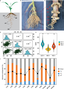
Supplement Figure 2 Distribution and correlation of root system architecture traits between each pair of locations. The significance levels of pairwise t-tests were added. * indicates P ≤ 0.05, ** indicates P ≤ 0.01; *** indicates P ≤ 0.001; **** indicates P ≤ 0.0001. Different lowercase letters indicate significant differences (P < 0.05) in different locations, as determined by Tukey's HSD test. Abbreviations for root traits are as follows: BRN, brace root number; BRWN, brace root whorl number; CR1, 1 st whorl crown roots; CR2, 2 nd whorl crown roots; CR3, 3 rd whorl crown roots; CR4, 4 th whorl crown roots; CR5, 5 th whorl crown roots; CR6, 6 th -8 th whorl crown roots; CRN, crown root number; CRWN, crown root whorl number; NRWN, nodal root whorl number. GX11: Guangxi location in 2011, HN11: Hainan location in 2011, YN11: Yunnan location in 2011. (TIF 9318 KB)

122_2023_4442_MOESM4_ESM.tif

Supplement Figure 3 The phenotypic distribution of root traits in the association panel. Abbreviations for root traits are as follows: BRN, brace root number; BRWN, brace root whorl number; CR1, 1 st whorl crown roots; CR2, 2 nd whorl crown roots; CR3, 3 rd whorl crown roots; CR4, 4 th whorl crown roots; CR5, 5 th whorl crown roots; CR6, 6 th -8 th whorl crown roots; CRN, crown root number; CRWN, crown root whorl number; NRWN, nodal root whorl number. (TIF 65415 KB)

122_2023_4442_MOESM5_ESM.tif

Supplement Figure 4 Phenotypic correlations among the root traits in the association panel. Abbreviations for root traits are as follows: BRN, brace root number; BRWN, brace root whorl number; CR1, 1 st whorl crown roots; CR2, 2 nd whorl crown roots; CR3, 3 rd whorl crown roots; CR4, 4 th whorl crown roots; CR5, 5 th whorl crown roots; CR6, 6 th -8 th whorl crown roots; CRN, crown root number; CRWN, crown root whorl number; NRWN, nodal root whorl number. (TIF 61613 KB)

122_2023_4442_MOESM6_ESM.tif

Supplement Figure 5 The percentage of total variance explained by each principal component. Abbreviations for root traits are as follows: BRN, brace root number; BRWN, brace root whorl number; CR1, 1 st whorl crown roots; CR2, 2 nd whorl crown roots; CR3, 3 rd whorl crown roots; CR4, 4 th whorl crown roots; CR5, 5 th whorl crown roots; CR6, 6 th -8 th whorl crown roots; CRN, crown root number; CRWN, crown root whorl number; NRN, nodal root number; NRWN, nodal root whorl number. (TIF 11460 KB)

122_2023_4442_MOESM7_ESM.tif

Supplement Figure 6 Comparison of root traits between PA and SPT heterotic groups. Different lowercase letters indicate significant differences ( P  < 0.05) in different locations, as determined by Tukey's HSD test. Abbreviations for root traits are as follows: BRN, brace root number; BRWN, brace root whorl number; CR1, 1 st whorl crown roots; CR2, 2 nd whorl crown roots; CR3, 3 rd whorl crown roots; CR4, 4 th whorl crown roots; CR5, 5 th whorl crown roots; CR6, 6 th -8 th whorl crown roots; CRN, crown root number; CRWN, crown root whorl number; NRN, nodal root number; NRWN, nodal root whorl number. (TIF 11656 KB)

122_2023_4442_MOESM8_ESM.tif

Supplement Figure 7 Quantile–quantile plots of root traits. (a) BRN, brace root number, (b) BRWN, brace root whorl number, (c) CR1, 1 st whorl crown roots, (d) CR2, 2 nd whorl crown roots, (e) CR3, 3 rd whorl crown roots, (f) CR4, 4 th whorl crown roots, (g) CR5, 5 th whorl crown roots, (h) CR6, 6 th -8 th whorl crown roots, (i) CRN, crown root number, (j) CRWN, crown root whorl number, (k) NRN, nodal root number, (l) NRWN, nodal root whorl number. (TIF 60252 KB)

Rights and permissions

Springer Nature or its licensor (e.g. a society or other partner) holds exclusive rights to this article under a publishing agreement with the author(s) or other rightsholder(s); author self-archiving of the accepted manuscript version of this article is solely governed by the terms of such publishing agreement and applicable law.

Reprints and permissions

About this article

Liu, Z., Li, P., Ren, W. et al. Hybrid performance evaluation and genome-wide association analysis of root system architecture in a maize association population. Theor Appl Genet 136 , 194 (2023). https://doi.org/10.1007/s00122-023-04442-7

Download citation

Received : 02 December 2022

Accepted : 04 August 2023

Published : 22 August 2023

DOI : https://doi.org/10.1007/s00122-023-04442-7

Share this article

Anyone you share the following link with will be able to read this content:

Sorry, a shareable link is not currently available for this article.

Provided by the Springer Nature SharedIt content-sharing initiative

• Find a journal
• Publish with us
• Track your research

An official website of the United States government

Here's how you know

Official websites use .gov A .gov website belongs to an official government organization in the United States.

Secure .gov websites use HTTPS A lock ( ) or https:// means you’ve safely connected to the .gov website. Share sensitive information only on official, secure websites.

•   Facebook
•   Twitter
•   Linkedin
•   Digg
•   Reddit
•   Pinterest
•   Email

Latest Earthquakes |    Chat Share Social Media  

Scientists discover genetically isolated populations and population-level inbreeding in a range-wide genetic analysis of the endangered rusty patched bumble bee

Range-wide genetic analysis of the endangered rusty patched bumble bee shows surprising levels of inbreeding within populations and genetic divergence between populations. Using a genetic mark-recapture technique, scientists also found lower site-level colony abundance than previously reported. 

Over the last three decades, the rusty patched bumble bee has disappeared from almost 90% of its former range. In 2017, it was federally listed as endangered under the U.S. Endangered Species Act. The genetic information generated through this study can inform managers in their conservation and restoration efforts of this endangered species.

Full citation: Mola, J.M., Pearse, I.S., Boone, M.L., Evans, E., Hepner, M.J., Jean, R.P., Kochanski, J.M., Nordmeyer, C., Runquist, E., Smith, T.A., Strange, J.P., Watson, J., Koch, J.B.U., 2024, Range-wide genetic analysis of an endangered bumble bee ( Bombus affinis,  Hymenoptera: Apidae) reveals population structure, isolation by distance, and low colony abundance,  Journal of Insect Science , v. 24, i. 2,  https://doi.org/10.1093/jisesa/ieae041 .

Related Content

Does the loss of plant diversity affect the health of native bees?

Loss of plant diversity is the primary cause of native bee decline. About 30-50% of all native bees are highly specialized, so if the plant they rely on disappears, the bees go away. If the bees disappear, the plant is unable to reproduce and dies out. While some of the plants pollinated by native bees are important food crops, other plants pollinated by native bees are critical for healthy...

How many species of native bees are in the United States?

There are over 20,000 known bee species in the world, and 4,000 of them are native to the United States. They range from the tiny (2 mm) and solitary Perdita minima , known as the world’s smallest bee, to kumquat-sized species of carpenter bees . Our bees come in as many sizes, shapes, and colors as the flowers they pollinate. There is still much that we don't know about native bees—many are...

What is the role of native bees in the United States?

About 75% of North American plant species require an insect—mostly bees—to move their pollen from one plant to another to effect pollination. Unlike the well-known behavior of the non-native honeybees, there is much that we don’t know about native bees. Many native bees are smaller in size than a grain of rice. Of approximately 4,000 native bee species in the United States, 10% have not been named...

Get Our News

These items are in the RSS feed format (Really Simple Syndication) based on categories such as topics, locations, and more. You can install and RSS reader browser extension, software, or use a third-party service to receive immediate news updates depending on the feed that you have added. If you click the feed links below, they may look strange because they are simply XML code. An RSS reader can easily read this code and push out a notification to you when something new is posted to our site.

Biology News

Ecosystems News

Fort Collins Science Center News

We've detected unusual activity from your computer network

To continue, please click the box below to let us know you're not a robot.

Why did this happen?

Please make sure your browser supports JavaScript and cookies and that you are not blocking them from loading. For more information you can review our Terms of Service and Cookie Policy .

For inquiries related to this message please contact our support team and provide the reference ID below.

Airline pilots at Delta, American, and United can make more than $500K a year — here's how their pay compares

• Recent pay raises have made commercial-airline pilots some of the highest-paid workers in the US.
• Three major airlines, American, Delta, and United, offer similar captain base pay of up to $447 an hour.
• Pilots can earn extras like bonuses and holiday pay, bringing some to half a million annually.

Commercial-airline pilots have become some of the highest-paid workers in the US thanks to a suite of post-pandemic pay raises .

American Airlines, Delta Air Lines , and United Airlines — which collectively employ nearly 50,000 pilots — have all signed lucrative contracts in recent years to attract and retain talent, and help with a lingering labor shortage . These pilots earn hundreds of dollars for every hour of flight time, with pay increasing with every year of seniority.

Across the board, the median airline pilot in the US earns just over $250,000 a year, according to the Bureau of Labor Statistics. Thanks to the recent pay bumps, combined with extra income opportunities like holiday pay and profit sharing, some pilots are taking home double that .

First officers, the typically less-experienced pilots who sit in the right seat, start at about $116 an hour at American and United, regardless of aircraft type, according to figures shared by the airlines. Those at Delta earn about $113.75 hourly across the fleet for the first year.

Every year that passes, a pilot gains seniority and a sizable pay bump.

Many of these pilots climb to captain on Airbus and Boeing wide-body planes and fly long-haul routes from their US hubs to cities in Europe and across the Americas. Some fly ultra-long-haul trips to places as far away as South Africa, Japan, and Australia.

Veterans at American and United in these categories will cap out around $500 an hour when their contracts expire in 2027. At Delta, they'll hit about $475 when their contract is up in 2026.

Profit sharing and bonuses can take their pay even higher

Pilot compensation is not only in the form of a base salary rate.

Each airline has its own packages with opportunities for extra pay, like profit sharing , bonuses, per diems, incentive rates, and holiday pay. Because the extra income is not always predictable because of operational reasons, it has not been included in this article.

Between base pay and extra incentives, the annual pay stubs are reading mid-six figures for the industry's most senior pilots.

Airline-pilot pay is complex, though, and depends on the pilot's seniority, their position, and the type of aircraft they fly, among other factors.

Not your usual 40-hour workweek

Airline pilots at American, Delta, and United are paid in " block time ," meaning they earn their full hourly rate only from gate to gate, earning per diems or other allowances to make up the work between flights.

Some pilots are paid to be on "reserve" when not scheduled to fly. These hours pay the same rate and have guaranteed minimums of 70 to 75 hours, depending on the airline, according to the Air Line Pilots Association .

For simplicity, the monthly and annual salary totals below are based on airline pilots who hold a "line," meaning they have a set month's schedule and are not on call. The ALPA said these pilots typically fly around 80 hours a month but can fly up to 100, per federal law .

Related stories

Here's a breakdown of the base pay pilots at American, Delta, and United earn per hour of payable time, according to contracts sent to Business Insider from the airline or its union. Salaries will increase over four years, but the base pay rates outlined for each airline reflect 2024.

American Airlines

First officers.

First-year first officer : about $116 an hour on any aircraft type.

12-year first officer : between $246 and $255 an hour on narrow-bodies and about $305 on wide-bodies.

A first-year first officer flying 80 hours each month would make about $9,300 monthly before taxes and other earnings, or about $111,000 yearly. That would jump to about $293,000 annually for a 12-year wide-body first officer.

First-year captain : between $331 and $340 an hour on narrow-bodies and about $410 on wide-bodies.

12-year captain: between $360 and $374 an hour on narrow-bodies and about $447 on wide-bodies.

A first-year captain flying 80 hours each month on most narrow-bodies would make about $26,500 monthly before taxes and other earnings, or about $318,000 yearly. That would jump to about $430,000 annually for a 12-year wide-body captain.

Delta Air Lines

First-year first officer : about $113.75 an hour on any aircraft type.

12-year first officer : between $216 and about $300 an hour, depending on the aircraft type.

A first-year first officer flying 80 hours each month would make about $9,100 monthly before taxes and other earnings, or about $109,000 yearly. That would jump to about $288,000 annually for a 12-year first officer on most of Delta's wide-bodies .

First-year captain : between $290 and about $402 an hour, depending on the aircraft type.

12-year captain : between $316 and about $438 an hour, depending on the aircraft type.

A first-year captain flying 80 hours each month on Delta's lowest-rate narrow-body, a Boeing 717, would make about $23,200 monthly before taxes and other earnings, or about $278,00 yearly. That would jump to about $420,000 yearly for a 12-year captain on most of Delta's wide-bodies.

United Airlines

12-year first officer : between $245 and about $305 an hour, depending on the aircraft type.

A first-year first officer flying 80 hours each month would make about $9,300 monthly before taxes and other earnings, or about $111,000 yearly. That would jump to about $293,000 annually for a 12-year first officer on most of United's wide-bodies.

First-year captain : between $329 and about $410 an hour, depending on the aircraft type.

12-year captain : between $358 and about $447 per hour, depending on the aircraft type.

A first-year captain flying 80 hours each month on United's lowest-end Airbus and Boeing narrow-bodies would make about $26,300 monthly before taxes and other earnings, or about $316,000 yearly. That would jump to about $429,000 yearly for a 12-year captain on most of United's wide-bodies .

Watch: Why flying is so terrible even though airlines spend billions

• Main content

An official website of the United States government

The .gov means it’s official. Federal government websites often end in .gov or .mil. Before sharing sensitive information, make sure you’re on a federal government site.

The site is secure. The https:// ensures that you are connecting to the official website and that any information you provide is encrypted and transmitted securely.

• Publications
• Account settings

Preview improvements coming to the PMC website in October 2024. Learn More or Try it out now .

• Advanced Search
• Journal List
• Front Genet

Sample Size for Successful Genome-Wide Association Study of Major Depressive Disorder

1 Department of Medical Science Mathematics, Medical Research Institute, Tokyo Medical and Dental University, Tokyo, Japan

2 CREST, JST, Tokyo, Japan

Hidenori Ochi

3 Division of Frontier Medical Science, Programs for Biomedical Research Graduate School of Biomedical Science, Department of Gastroenterology and Metabolism, Hiroshima University, Hiroshima, Japan

4 Laboratory for Digestive Diseases, RIKEN Center for Integrative Medical Sciences, Hiroshima, Japan

5 Laboratory for Autoimmune Diseases, RIKEN Center for Integrative Medical Sciences, Yokohama, Japan

Tatsuhiko Tsunoda

6 Laboratory for Medical Science Mathematics, RIKEN Center for Integrative Medical Sciences, Yokohama, Japan

7 Risk Analysis Research Center, The Institute of Statistical Mathematics, Tachikawa, Tokyo, Japan

Shigeyuki Matsui

8 Department of Biostatistics, Nagoya University Graduate School of Medicine, Nagoya, Japan

Associated Data

Major depressive disorder (MDD) is a complex, heritable psychiatric disorder. Advanced statistical genetics for genome-wide association studies (GWASs) have suggested that the heritability of MDD is largely explained by common single nucleotide polymorphisms (SNPs). However, until recently, there has been little success in identifying MDD-associated SNPs. Here, based on an empirical Bayes estimation of a semi-parametric hierarchical mixture model using summary statistics from GWASs, we show that MDD has a distinctive polygenic architecture consisting of a relatively small number of risk variants (~17%), e.g., compared to schizophrenia (~42%). In addition, these risk variants were estimated to have very small effects (genotypic odds ratio ≤ 1.04 under the additive model). Based on the estimated architecture, the required sample size for detecting significant SNPs in a future GWAS was predicted to be exceptionally large. It is noteworthy that the number of genome-wide significant MDD-associated SNPs would rapidly increase when collecting 50,000 or more MDD-cases (and the same number of controls); it can reach as much as 100 SNPs out of nearly independent (linkage disequilibrium pruned) 100,000 SNPs for ~120,000 MDD-cases.

Introduction

Major depressive disorder (MDD) is a common, complex disorder with a high lifetime prevalence of ~15% (Kessler et al., 2003 ) and a moderate heritability of 31–42% (Sullivan et al., 2000 ). Etiological understanding of MDD is potentially of great impact on individuals and public health. Several statistical genetics approaches have suggested that a large portion of the heritability of MDD is explained by common single nucleotide polymorphisms (SNPs) (Lubke et al., 2012 ; Lee et al., 2013 ). However, no significant MDD-associated variant has been discovered even in a large genome-wide association study (GWAS) with around 9,500 cases by the Psychiatric Genomics Consortium (PGC) (Major Depressive Disorder Working Group of the Psychiatric Genomics Consortium, 2013 ; Levinson et al., 2014 ). Most recently, two studies have respectively identified one genome-wide significant SNP for particular subpopulations with relatively less phenotypic heterogeneity. One used severe Han Chinese women patients (Cai et al., 2015 ) and the other reanalyzed the data collected from the PGC with stratification by self-reported age (Power et al., 2017 ). In contrast, as a GWAS analysis for a general population without restriction to particular subpopulations, Hyde et al. ( 2016 ) used European self-reported phenotyped data from a consumer genomics company, 23andMe, composed of a massive sample size of 75,607 cases and 231,747 controls, and identified 15 independent loci associated with major depression. However, one possible limitation of this study is the validity of self-reported phenotype information. Therefore, although it provided a candidate list of disease-associated loci for the first time, further GWASs are warranted for discovery of new variants associated with MDD.

The power to discover new disease-associated variants critically depends on the underlying genetic architecture, i.e., the number of risk loci and their frequencies and effect sizes. One possible reason for the difficulty in identifying variants associated with MDD might relate to the disease's high prevalence/low heritability feature. Based on these perspectives, Wray et al. ( 2012 ) carefully quantified that sample sizes 4 to 5-fold greater are needed for GWASs of MDD compared with schizophrenia (SCZ), assuming the same number and frequency of risk variants underlying SCZ and MDD.

In this study, utilizing GWAS summary data of PGC (Major Depressive Disorder Working Group of the Psychiatric Genomics Consortium, 2013 ), we unbiasedly estimated the proportion of disease-associated variants and their effect size distribution with the use of our recently developed empirical Bayes method with a semi-parametric hierarchical mixture model (SP-HMM) (Nishino et al., 2018 ). Based on the estimated genetic architectures by this method, we explain why GWASs of MDD have failed to discover disease-associated variants, through comparisons with other diseases, including SCZ (Ripke et al., 2014 ), type 2 diabetes (T2D) (Morris et al., 2012 ) with similar heritability and prevalence to MDD, and Crohn's disease (CD) (Liu et al., 2015 ), for which GWASs to date have successfully identified disease-associated variants. We also analyzed GWAS data for other psychiatric disorders including autism spectrum disorders (ASDs) (Autism Spectrum Disorder Working Group of the Psychiatry Genomics Consortium, 2015 ) and anorexia nervosa (AN) (Boraska et al., 2014 ), which have not had much progress in GWAS. We then predicted a curve of the number of significant SNPs or the number of new discoveries for various sizes of future GWASs. This prediction would be particularly useful for designing future GWASs for complex diseases for which limited disease-associated variants have been identified.

Proportion of disease-associated SNPs and their effect-size distributions

We obtained nearly independent pruned SNP sets consisting of around m = 100,000 SNPs for the six GWASs (Table S1 ). The SP-HMM was fitted to each pruned SNP set to estimate the proportion of disease-associated SNPs, π, and their effect size distribution, g , non-parametrically (Figure ​ (Figure1). 1 ). The proportion of disease-associated SNPs, π, for SCZ was estimated to be the largest ( π ^   ~   42 . 2   % ), i.e., SCZ was highly polygenic, followed by T2D and CD. ASDs was the least polygenic ( π ^   ~   9 . 4   % ) among the six GWASs. MDD was the second least polygenic, π ^   ~   17 . 0   % . For AN, π was estimated to be intermediate, π ^   ~   21 . 3   % .

Estimated proportions of disease-associated SNPs, π ^ , and effect-size distributions for disease-associated SNPs, ĝ. π ^ corresponds to the areas under the curves. Numbers after the plus-minus signs (“±”) are standard errors by 100 parametric bootstrap samples based on the estimated SP-HMM. Vertical allows in the figures indicate small peaks with relatively large effects.

Non-parametric estimation of g flexibly characterized the effect-size distributions for the six diseases as follows. A noteworthy feature in the effect-size distribution of disease-associated SNPs, g , for MDD is that there were few SNPs with large effects; most were within |β| = 0.03 (genotypic odds ratio = 1.03 under the additive model) and almost all SNPs were within |β| = 0.04 (odds ratio = 1.04). For ASDs, effect sizes were estimated to be relatively small among the six GWASs; almost all SNPs were within |β| = 0.05. For CD, we had many disease-associated SNPs with effect sizes near or more than |β| = 0.05 or odds ratio = 1.05, and also peaks of effects around |β| = 0.1. The estimated distribution of g for SCZ lay mostly within a range of |β| ≤ 0.03, but with peaks at relatively large effects of |β| 0.05 or larger. AN had relatively large effects, particularly in the positive signed region. For T2D, while most disease-associated SNPs were within |β| = 0.03, there was a small portion of disease-associated SNPs with the effect sizes near or more than |β| = 0.05.

Prediction of the number of significant SNPs

Figure ​ Figure2 2 shows the predicted number of significant SNPs, K ^ , with the genome-wide significance level of p c = 5 × 10 −8 (Figure ​ (Figure2A) 2A ) and suggestive level of p c = 1 × 10 −6 (Figure ​ (Figure2B) 2B ) for each disease, assuming m * = 100,000 independent SNPs in a future GWAS. Also, Figure S1 shows K ^ with 95% confidence intervals for each disease in log scale. We first confirmed that the observed number of significant SNPs in the pruned SNP sets in the current GWASs, shown in dots, was well-captured by the predicted curves in all the diseases. In both levels of the statistical significance thresholds, the number of significant SNPs was predicted to be by far the largest for CD in all ranges of the effective number of cases. The predicted number of statistical significance was the second largest for SCZ. Those for AN were next to and near those for SCZ. For detecting 1, 10, and 100 genome-wide significant SCZ-associated SNPs, 7,000, 18,000, and 51,000 effective number of cases was predicted to be needed, respectively. We observed that, for MDD, the predicted number of statistically significant SNPs was exceptionally small in both levels of the statistical significance thresholds (Figure ​ (Figure2). 2 ). Nevertheless, the predicted number for MDD rapidly increases when n e * > 50,000. For detecting 1, 10, and 100 genome-wide significant MDD-associated SNPs, 34,000, 61,000, and 118,000 effective number of cases was predicted to be needed, respectively (Figure S2 ). For detecting 1, 10, and 100 genome-wide significant SCZ-associated SNPs, 7,000, 18,000, and 51,000 effective number of cases was predicted to be needed (Figure S2 ), which was 4.9, 3.4, and 2.3 times larger than those for SCZ, respectively. Those numbers were 4.9, 3.4, and 2.3 times larger than those for SCZ, respectively. For ASDs, the predicted curves of the number of disease-associated SNPs with significance in both levels of statistical significance thresholds lay in the middle of those for SCZ and MDD (Figure ​ (Figure2). 2 ). For T2D, in case of n e * < 2,000, the number of detected SNPs was predicted to be close to those for SCZ and AN. However, as the sample size increased, the predicted detections for T2D with the genome-wide significance and suggestive level became smaller than those for ASDs, or even for MDD.

Predicted number of significant SNPs, K ^ , under the estimated SP-HMM. Predicted number of significant SNPs, K ^ , was calculated assuming m * = 100,000 independent SNPs in the “future” GWASs. Dots show observed values in the pruned SNP sets of current GWAS data. (A) Genome-wide significance level: p c = 5 × 10 −8 . (B) Genome-wide suggestive level: p c = 10 −6 .

Although GWASs have played a critical role in discovering disease-associated variants for many complex diseases, this approach has not necessarily worked well for some diseases, including psychiatric disorders such as MDD. In this paper, we have attempted to explain the reason for the failure in GWASs for such diseases, through estimating the genetic architecture based on an empirical Bayes estimation of a flexible, semi-parametric hierarchical mixture model (Nishino et al., 2018 ) using summary data from the existing GWASs (Figure ​ (Figure1 1 ).

For the six diseases examined, we commonly observed that the genetic basis consisted of enormous variants, ranging from π ^   ~ 9.4 to 42.2% in the nearly independent 100,000 genome-wide SNPs, with small effects (majority of genotypic odds ratio for risk alleles are within 1.05 under the additive model). In regard to MDD, the SP-HMM clarified the distinctive feature of polygenicity; the proportion of MDD-associated SNPs was relatively small, π ^   ~   17 . 0   % compared with other diseases (SCZ, T2D, CD, ASDs, and AN), and the absolute effect sizes for almost all of the non-null SNPs were very small, |β| ≤ 0.04, in the pruned GWAS data from PGC (Major Depressive Disorder Working Group of the Psychiatric Genomics Consortium, 2013 ) (Figure ​ (Figure1 1 ).

However, this difficulty in discovering MDD-associated variants can be addressed with increased sample sizes. A prediction on the number of discoveries in a future GWAS based on the estimated genetic architecture indicated that the number of significant SNPs can substantially increase when collecting 50,000 or more MDD-cases (and the same number of controls). It can reach as much as 100 SNPs out of 100,000 independent SNPs for ~120,000 MDD-cases (Figure ​ (Figure2 2 and Figure S2 ). Note that the results cannot rule out the importance of taking into account rare variants, environment-gene interaction (Caspi et al., 2010 ), and heterogeneity possibly resolved by stratified analysis (Power et al., 2017 ).

One reviewer of this article kindly informed us that the MDD-PGC group identified 44 independent significant SNPs using the seven cohorts (130,664 cases and 330,470 controls in total) including PGC data with 16,823 cases and 25,632 controls (Wray et al., 2018 ). One part of the results of that study seems to be consistent with our estimate that the effect sizes of MDD-associated SNPs were very small, i.e., |β| ≤ 0.04 (Figure ​ (Figure1); 1 ); the crude odds ratio estimates of 41 SNPs of 44 significant SNPs in the PGC (2017) were 0.96, 0.97, 1.03, or 1.04, that is | β ^ | ≤ 0 . 04 (Table 1 in Wray et al., 2018 ). Note that the true effect sizes of the 44 SNPs would be generally smaller than those of estimates, as the crude estimate is subject to the “winners curse.” On the other hand, by the present method, the number of significant SNPs assuming 100,000 independent SNPs was predicted as 355.1 (95% confidence interval 239.7–683.3) using the sample with 130,664 cases and 330,470 controls, which largely exceeded the observed number, 44 (Figure S1 ). (Note that our estimation targeting 100,000 independent SNPs is supposed to underestimate the number of significant SNPs seen in practical situations, where SNPs with higher association (e.g., lower P -value) are preferentially selected among “all SNPs” so that linkage disequilibrium (LD) among selected SNPs are nearly independent). The discrepancy between our prediction and the observation could be due to the difference between the PGC cohort data and data from the other six cohorts, especially, self-reported data from 23andMe with 130,664 cases and 330,470 controls, which accounted for the large proportion of the total cohorts. In fact, the SNP heritability estimates in observed scales were much smaller for 23andMe data (0.038) than for PGC data (0.128) (Hyde et al., 2016 ). Our over prediction suggests that for MDD, possibly for other diseases, phenotyping methods have great impact on the number of significant SNPs. Despite the reduced power, self-reported data from a consumer genomics company, e.g., 23andMe, would increase in importance due to its utility. It is our intention to clarify the difference in effect-size of disease-associated variants between self-reported data and established phenotyped data.

In addition to MDD, the prediction analysis can be used for comparing the number of discoveries among diseases. For example, the number of future discoveries for AN is expected to be of the same extent as for SCZ, while the number for ASDs is predicted to be intermediate between those for SCZ and MDD.

Using a method similar to the present study, Park et al. ( 2010 ) investigated the relationship between sample size and the number of significant disease-associated SNPs based on the estimated effect size distribution of disease-associated SNPs. This method, however, is limited to relatively large effect sizes in the effect-size estimation due to the need to use SNPs with some significant level, and requires adjustment for the winner's curse (selection bias in using top significant SNPs) in the estimation. Stahl et al. ( 2012 ) proposed a method to estimate the proportion of disease-associated SNPs and the effect-size distribution using an approximate Bayesian polygenic analysis (ABPA). The application to evaluate the relationship between sample size and the number of significant disease-associated SNPs has been limited to few studies because of technical complexity and excess computational burden with many simulations (to our knowledge, Ripke et al., 2013 applied the ABPA method). There are also several “Gaussian mixture models” to estimate the underlying effect sizes using the z-scores for SNPs as the inputs (Thompson et al., 2015 ; Holland et al., 2016 ). These models are applicable to investigate the relationship between sample size and the number of significant disease-associated SNPs, although the authors did not directly study this problem. Note that the definitions of effect sizes in the above existing methods are different from that of the SP-HMM, e.g., 2 f (1− f )β 2 for Park et al. ( 2010 ), and 2 f ( 1 - f ) β for Thompson et al. ( 2015 ), where f is the allele frequency.

The features of the SP-HMM make it quick and easy to compute the number of significant disease-associated SNPs given sample sizes understanding the estimated proportion of the disease-associated SNPs and effect-size distribution where the effect size is easy to understand, defined as the genotype log-odds ratio under the additive model, β. In making inference about a SNP regarding its null/non-null association with disease status, the number of components, in principle, is two (i.e., null and non-null components). In modeling the non-null component (effect size distribution), the parametric approach, e.g., finite normal mixture models with several components, is a popular choice. Unlike such a parametric model, we assume a non-parametric distribution as a “single” non-null component to cover all such non-null components. This is the interpretation for the modeling formula given in the subsection “Semi-parametric Hierarchical Mixture Model (SP-HMM)” in the Materials and Methods section. Meanwhile, in estimation using the expectation–maximization (EM) algorithm we can see our model as that with “so many” non-null components (the number of components = B , described in the subsection “Semi-parametric Hierarchical Mixture Model (SP-HMM)” in the discretized effect size distribution used in the estimation algorithm). We have shown that with 3–5,000 or more cases (and the same number of controls), the estimates of π and g are fairly accurate, leading to reliable estimates of the number of significant disease-associated SNPs (Nishino et al., 2018 ). Note that our prediction of the number of significant SNPs targets “the LD-pruned SNP set” in the future GWAS data, where SNPs would be randomly selected so that LDs among SNPs should be r 2 < 0.1. This limitation regarding the target SNPs (i.e., the LD-pruned SNP set) will be addressed in future work. Although we assumed 100,000 SNPs in the LD-pruned set from the observations in Table S1 , a different number of SNPs in the LD-pruned set would be considered in the proposed approach. This is because the number should depend on the effective size of study population, as is the case for “the effective number of chromosome segments” ( M e ; the key determinant of the accuracy of genomic prediction) does, i.e., M e = 2.938 N e 0 . 965 under 30 Morgan in total, where N e is the effective population size (Lee et al., 2017 ).

In conclusion, our prediction analysis is generally useful for designing future GWASs for complex diseases, through estimating additional number of cases (and controls) needed to be collected in a single cohort study, or additional cohorts (sample sets) needed to be included in a meta-analysis, and for discovering a given number of new disease-associated variants.

Materials and methods

Semi-parametric hierarchical mixture model (sp-hmm).

To estimate polygenic architectures of the six diseases, we used the SP-HMM (Nishino et al., 2018 ). The SP-HMM estimates the proportion of disease-associated SNPs, π, and their effect size distribution, g , non-parametrically, using GWAS summary statistics on effect sizes (genotype log-odds ratios) which often are available through Web sites. The “non-parametric estimation of g ” enables us to flexibly characterize the effect-size distributions without any assumptions for forms of the distribution. The SP-HMM assumes independence among SNPs, as was justified by pruning SNP described below. The SP-HMM has been validated through various types of polygenic scenarios and the required sample size was confirmed to be around 3–5,000 or more (see Nishino et al., 2018 for more details about the SP-HMM). The SP-HMM is briefly described in the following.

Letting a and A be the derived and ancestral alleles status, respectively. The genotypes AA , Aa , and aa in each SNP assumed to have dosages x j = 0, 1, and 2, respectively. Under the additive allele dosage model, we defined the effect size, β j , as the genotype log-odds ratio for the j -th SNP of the total m SNPs. The estimate of β j was denoted by Y j = β ^ j . For Y j 's, a two-component mixture model with null and non-null SNPs components is assumed:

where f 0 j and f 1 j are the probability densities for null and non-null SNPs, respectively, and π is the probability of being non-null. Let V ^ β ^ j be an empirical variance estimate of β ^ j . Asymptotic distribution of β ^ j were assumed. For null SNPs, we specified y j   ~   f 0 j ( y j ) = N ( 0 , V ^ β ^ j ) . For non-null SNPs, we assumed the hierarchical structure: y j | β j   ~   f 1 j ( y j | β j ) = N ( β j , V ^ β ^ j ) and β j ~ g , where the effect-size distribution g is unspecified. We regard this model as a semi-parametric model, as the standard asymptotic normality is assumed for β ^ j at the individual SNP level, while its true effect size β j follows a non-parametric prior distribution g . The assumption of independence among y j 's would be reasonable for a set of LD-pruned SNPs (for the details about pruning see the subsection of “GWAS Data”). We estimated the priors, π and g , based on the data by applying an expectation–maximization (EM) algorithm, that is, empirical Bayes estimation. The non-parametric estimate of g was discrete with mass points p = ( p 1 , p 2 , …, p B ) at a series of nonzero points b = ( b 1 , b 2 , …, b B ) ( b 1 < b 2 < ··· < b B ). We set b 1 = −0.3 and b B = 0.3 (0.74 and 1.35 in odds ratio). The number grid point B = 120 was used, such that b = (−0.300, −0.295, …, −0.005, 0.005, …, 0.295, 0.300). The initial value of π and the initial distribution of g were important and determined by a careful procedure (for details, see Nishino et al., 2018 ). To estimate standard errors of π ^ and 95% confidence interval of K ^ , the parametric bootstrap method based on the estimated SP-HMM was used. The validity of the estimation using the SP-HMM has been demonstrated via an extensive simulation experiment under various scenarios in terms of sample size, π, g , and possible correlations among SNP (Nishino et al., 2018 ).

For the j -th SNP, the power to detect an association with effect size β j , Power j (β j ), is given by

where Φ μ, 1 (·) denotes the cumulative distribution function of the normal distribution with mean μ and unit variance, and z c denotes the rejection threshold determined by a significance level, p c , satisfying z c = Φ 0 , 1 - 1 ( 1 - p c / 2 ) ). In this study, p c = 5 × 10 −8 (the genome-wide “significant” threshold) and p c = 1 × 10 −6 (the genome-wide “suggestive” threshold) were used. Under the SP-HMM, the rejection probability, i.e., the probability that the j -th SNP is significant, is given by

Let n r and n s be the sample sizes for cases and controls, respectively, in an existing GWAS from which we can estimate the SP-HMM. In addition, we envisage a “future” GWAS with n r * cases and n s * controls. Based on the formula (1), the probability of significance for the j -th SNP in the future GWAS can be obtained through replacing V ^ β ^ j with V ^ β ^ j × 1/(1/ n r + 1/ n s ) × (1/ n r * + 1/ n s * ), since the empirical variance of β ^ j is approximately proportional to the sum of inverses of case and control sample sizes. This approximation has been used in the GWAS meta-analysis (Willer et al., 2010 ). The derivation in the logistic regression for “large sample and small effect-size” limit was done elsewhere (e.g., by Lin and Sullivan, 2009 ). The number of significant SNPs, K , in the future data set consisting of m * SNPs is then predicted as

where P ¯ is the average rejection probability over all SNPs in the SNP set, P ¯ = ∑ j = 1 m P j / m , replacing V ^ β ^ j with V ^ β ^ j × 1/(1/ n r + 1/ n s ) × (1/ n r * + 1/ n s * ), π with π ^ and g with ĝ, respectively, in the formula (1). We set m * = 100,000 for targeting 100,000 pruned SNPs. Since the term (1/ n r * + 1/ n s * ) determines the predicted number of significant SNPs, K ^ , we define the “effective number of cases” as n e * = 2 / ( 1 / n r * + 1 / n s * ) . As such, we can obtain a curve of the number of significant SNPs in a future GWAS, K ^ , as a function of its sample size, n e * , based on the estimated SP-HMM using the existing GWAS data.

The six sets of GWAS summary statistics for MDD (Major Depressive Disorder Working Group of the Psychiatric Genomics Consortium, 2013 ), SCZ (Ripke et al., 2014 ), T2D (Morris et al., 2012 ), CD (Liu et al., 2015 ), ASDs (Autism Spectrum Disorder Working Group of the Psychiatry Genomics Consortium), and AN (Boraska et al., 2014 ) were used, which are all available online (MDD, SCZ, ASDs and AN, www.med.unc.edu/pgc/downloads ; T2D, http://www.diagram-consortium.org/ ; IBD, http://www.ibdgenetics.org/downloads.html ; see Table S1 for sample size). To restrict analysis to well-imputed, high-quality variants, we used only SNPs that existed on the HapMap 3 reference panel (International HapMap 3 Consortium., 2010 ). For the pruned SNP sets, we included SNPs randomly, irrespective of degrees of association such that no SNPs in the set were in r 2 > 0.1, as done in the previous work (Nishino et al., 2018 ). We selected one SNP randomly from all the SNP data and SNPs in LD ( r 2 > 0.1) with the selected SNP removed. This was repeated until no SNPs remained. LD information( r 2 ) was extracted from the HapMap database (HapMap phases I+II+III, release 27) (International HapMap 3 Consortium., 2010 ). With this pruning process, we could interpret the significant SNPs as SNPs linked to independent causal variants. Meanwhile, the SP-HMM analysis evaluates the marginal effect of the pruned SNPs and underestimates the effects of causal variants; estimated effect-size distributions should be smaller than those of causal variants, and the estimates π ^ × (the number of SNPs in the SNP sets) would give conservative estimates of the number of causal variants. Nevertheless, the SP-HMM estimation reflects the effects of the causal variants for each disease through linkage disequilibrium. LD information was retrieved from the HapMap (International HapMap 3 Consortium., 2010 ) data base (HapMap phases I+II+III, release 27). The ancestral/derived alleles for each SNP were determined from dbSNP (Nishino et al., 2018 ). We calculated the estimate of log-odds ratio for the j -th SNP, β ^ j , and its variance, V ^ β ^ j for applying the SP-HMM to the pruned SNP sets and predicting of number of significant SNPs.

Empirical validation for prediction of the number of significant SNPs

We validated our approach for predicting the number of significant SNPs using hypothetical “current” and “future” GWAS data; we fitted the SP-HMM to the “current” GWAS data with smaller sample size to predict the number of significant SNPs in the “future” GWAS data with larger sample size, and we compared the predicted value with the observed one. The three pairs of GWAS summary statistics for SCZ (for “current” data, Cross-Disorder Group of the Psychiatric Genomics Consortium, 2013 ; for “future” data, Major Depressive Disorder Working Group of the Psychiatric GWAS Consortium, 2013), bipolar disorder (for 'current' data, Cross-Disorder Group of the Psychiatric Genomics Consortium, 2013 ; for 'future' data, Ripke et al., 2014 ), and coronary artery disease (for “current” data, The Coronary Artery Disease (C4D) Genetics Consortium, 2011 ; for “future” data, Schunkert et al., 2011 ) are all available online (SCZ, bipolar disorder, www.med.unc.edu/pgc/downloads ; coronary artery disease, www.cardiogramplusc4d.org/data-downloads/ ). The quality control and pruning for the SNP data were done as described in the previous subsection, “GWAS Data.” For SCZ, bipolar disorder, and coronary artery disease, there were 101314, 96681, and 79512 SNPs in the pruned sets, respectively. Those values were set as m * in the formula (2). The number of SNPs was smaller for coronary artery disease (79512), as the original GWAS summary data have been imputed using HapMap data. Table S2 shows the validation results. The observed number of significant SNPs for each disease was well-predicted by our approach.

Author contributions

JN and SM: Conceptualization; JN: Formal analysis; TT and SM: Funding acquisition; JN and SM: Writing original draft; HO, YK and TT: Writing review and editing.

Conflict of interest statement

The authors declare that the research was conducted in the absence of any commercial or financial relationships that could be construed as a potential conflict of interest.

Acknowledgments

This study made use of data generated by International Inflammatory Bowel Disease Genetics Consortium (IIBDGC), DIAbetes Genetics Replication and Meta-analysis (DIAGRAM), and Psychiatric Genomic Consortium (PGC).

Funding. We thank a Grant-in-Aid for Scientific Research (16H06299) and JST- CREST (JPMJCR1412) from the Ministry of Education, Culture, Sports, Science and Technology of Japan.

Supplementary material

The Supplementary Material for this article can be found online at: https://www.frontiersin.org/articles/10.3389/fgene.2018.00227/full#supplementary-material

• Autism Spectrum Disorder Working Group of the Psychiatry Genomics Consortium (2015). Dataset: PGC-ASD Summary Statistics From a Meta-Analysis of 5,305 ASD-Diagnosed Cases and 5,305 Pseudocontrols of European Descent (Based on Similarity to CEPH Reference Genotypes) . Available online at: http://www.med.unc.edu/pgc/results-anddownloads .
• Boraska V., Franklin C. S., Floyd J. A., Thornton L. M., Huckins L. M., Southam L., et al.. (2014). A genome-wide association study of anorexia nervosa . Mol. Psychiatry 19 , 1085–1094. 10.1038/mp.2013.187 [ PMC free article ] [ PubMed ] [ CrossRef ] [ Google Scholar ]
• Cai N., Bigdeli T. B., Kretzschmar W., Li Y. H., Liang J. Q., Song L., et al. (2015). Sparse whole-genome sequencing identifies two loci for major depressive disorder . Nature 523 , 588–591. 10.1038/nature14659 [ PMC free article ] [ PubMed ] [ CrossRef ] [ Google Scholar ]
• Caspi A., Sugden K., Moffitt T. E., Taylor A., Craig I. W., Harrington H., et al.. (2010). Influence of life stress on depression: moderation by a polymorphism in the 5-HTT gene . Science 301 , 386–389. 10.1126/science.1083968 [ PubMed ] [ CrossRef ] [ Google Scholar ]
• Coronary Artery Disease (C4D) Genetics Consortium Consortium. (2011). A genome-wide association study in Europeans and South Asians identifies five new loci for coronary artery disease . Nat. Genet . 43 , 339–344. 10.1038/ng.782 [ PubMed ] [ CrossRef ] [ Google Scholar ]
• Cross-Disorder Group of the Psychiatric Genomics Consortium (2013). Identification of risk loci with shared effects on five major psychiatric disorders: a genome-wide analysis . Lancet 381 , 1371–1379. 10.1016/S0140-6736(12)62129-1 [ PMC free article ] [ PubMed ] [ CrossRef ] [ Google Scholar ]
• Holland D., Wang Y., Thompson W. K., Schork A., Chen C. H., Lo M. T., et al.. (2016). Estimating effect sizes and expected replication probabilities from GWAS summary statistics . Front. Genet. 7 :15. 10.3389/fgene.2016.00015 [ PMC free article ] [ PubMed ] [ CrossRef ] [ Google Scholar ]
• Hyde C. L., Nagle M. W., Tian C., Chen X., Paciga S. A., Wendland J. R., et al.. (2016). Identification of 15 genetic loci associated with risk of major depression in individuals of European descent . Nat. Genet. 48 , 1031–1036. 10.1038/ng.3623 [ PMC free article ] [ PubMed ] [ CrossRef ] [ Google Scholar ]
• International HapMap 3 Consortium (2010). Integrating common and rare genetic variation in diverse human populations . Nature 467 , 52–58. 10.1038/nature09298 [ PMC free article ] [ PubMed ] [ CrossRef ] [ Google Scholar ]
• Kessler R., Berglund P., Demler O., Jin R., Koretz D., Merikangas K., et al. (2003). The epidemiology of major depressive disorder . J. Am. Med. Assoc. 23 , 3095–3105. 10.1001/jama.289.23.3095 [ PubMed ] [ CrossRef ] [ Google Scholar ]
• Lee S. H., Clark S., Van Der Werf J. H. J. (2017). Estimation of genomic prediction accuracy from reference populations with varying degrees of relationship . PLoS ONE 12 :e0189775. 10.1371/journal.pone.0189775 [ PMC free article ] [ PubMed ] [ CrossRef ] [ Google Scholar ]
• Lee S. H., Ripke S., Neale B. M., Faraone S. V., Purcell S. M., Perlis R. H., et al.. (2013). Genetic relationship between five psychiatric disorders estimated from genome-wide SNPs . Nat. Genet. 45 , 984–994. 10.1038/ng.2711 [ PMC free article ] [ PubMed ] [ CrossRef ] [ Google Scholar ]
• Levinson D. F., Mostafavi S., Milaneschi Y., Rivera M., Ripke S., Wray N. R., et al.. (2014). Genetic studies of major depressive disorder: why are there no genome-wide association study findings and what can we do about it? Biol. Psychiatry 76 , 510–512. 10.1016/j.biopsych.2014.07.029 [ PMC free article ] [ PubMed ] [ CrossRef ] [ Google Scholar ]
• Lin D. Y., Sullivan P. F. (2009). Meta-analysis of genome-wide association studies with overlapping subjects . Am. J. Hum. Genet. 85 , 862–872. 10.1016/j.ajhg.2009.11.001 [ PMC free article ] [ PubMed ] [ CrossRef ] [ Google Scholar ]
• Liu J. Z., van Sommeren S., Huang H., Ng S. C., Alberts R., Takahashi A., et al.. (2015). Association analyses identify 38 susceptibility loci for inflammatory bowel disease and highlight shared genetic risk across populations . Nat. Genet. 47 , 979–989. 10.1038/ng.3359 [ PMC free article ] [ PubMed ] [ CrossRef ] [ Google Scholar ]
• Lubke G. H., Hottenga J. J., Walters R., Laurin C., De Geus E. J. C., Willemsen G., et al.. (2012). Estimating the genetic variance of major depressive disorder due to all single nucleotide polymorphisms . Biol. Psychiatry 72 , 707–709. 10.1016/j.biopsych.2012.03.011 [ PMC free article ] [ PubMed ] [ CrossRef ] [ Google Scholar ]
• Major Depressive Disorder Working Group of the Psychiatric Genomics Consortium (2013). A mega-analysis of genome-wide association studies for major depressive disorder . Mol. Psychiatry 18 , 497–511. 10.1038/mp.2012.21 [ PMC free article ] [ PubMed ] [ CrossRef ] [ Google Scholar ]
• Morris A. P., Voight B. F., Teslovich T. M., Ferreira T., Segrè A. V., Steinthorsdottir V., et al.. (2012). Large-scale association analysis provides insights into the genetic architecture and pathophysiology of type 2 diabetes . Nat. Genet. 44 , 981–990. 10.1038/ng.2383 [ PMC free article ] [ PubMed ] [ CrossRef ] [ Google Scholar ]
• Nishino J., Kochi Y., Shigemizu D., Kato M., Ikari K., Ochi H., et al.. (2018). Empirical Bayes estimation of semi-parametric hierarchical mixture models for unbiased characterization of polygenic disease architectures . Front. Genet. 9 :115. 10.3389/fgene.2018.00115 [ PMC free article ] [ PubMed ] [ CrossRef ] [ Google Scholar ]
• Park J.-H. H., Wacholder S., Gail M. H., Peters U., Jacobs K. B., Chanock S. J., et al.. (2010). Estimation of effect size distribution from genome-wide association studies and implications for future discoveries . Nat. Genet. 42 , 570–575. 10.1038/ng.610 [ PMC free article ] [ PubMed ] [ CrossRef ] [ Google Scholar ]
• Power R. A., Tansey K. E., Buttenschon H. N., Cohen-Woods S., Bigdeli T., Hall L. S., et al.. (2017). Genome-wide association for major depression through age at onset stratification: major depressive disorder working group of the psychiatric genomics consortium . Biol. Psychiatry 81 , 325–335. 10.1016/j.biopsych.2016.05.010 [ PMC free article ] [ PubMed ] [ CrossRef ] [ Google Scholar ]
• Ripke S., Neale B. M., Corvin A., Walters J. T. R., Farh K.-H., Holmans P. A., et al. (2014). Biological insights from 108 schizophrenia-associated genetic loci . Nature 511 , 421–427. 10.1038/nature13595 [ PMC free article ] [ PubMed ] [ CrossRef ] [ Google Scholar ]
• Ripke S., O'Dushlaine C., Chambert K., Moran J. L., Kahler A. K., Akterin S., et al.. (2013). Genome-wide association analysis identifies 13 new risk loci for schizophrenia . Nat. Genet. 45 , 1150–1159. 10.1038/ng.2742 [ PMC free article ] [ PubMed ] [ CrossRef ] [ Google Scholar ]
• Schunkert H., Konig I. R., Kathiresan S., Reilly M. P., Assimes T. L., Holm H., et al.. (2011). Large-scale association analysis identifies 13 new susceptibility loci for coronary artery disease . Nat. Genet. 43 , 333–338. 10.1038/ng.784 [ PMC free article ] [ PubMed ] [ CrossRef ] [ Google Scholar ]
• Stahl E. A., Wegmann D., Trynka G., Gutierrez-Achury J., Do R., Voight B. F., et al.. (2012). Bayesian inference analyses of the polygenic architecture of rheumatoid arthritis . Nat. Genet. 44 , 483–489. 10.1038/ng.2232 [ PMC free article ] [ PubMed ] [ CrossRef ] [ Google Scholar ]
• Sullivan P. F., Neale M. C., Kendler K. S. (2000). Genetic epidemiology of major depression : review and meta-analysis . Am. J. Psychiatry 157 , 1552–1562. 10.1176/appi.ajp.157.10.1552 [ PubMed ] [ CrossRef ] [ Google Scholar ]
• Thompson W. K., Wang Y., Schork A. J., Witoelar A., Zuber V., Xu S., et al.. (2015). An empirical Bayes mixture model for effect size distributions in genome-wide association studies . PLoS Genet. 11 :e1005717. 10.1371/journal.pgen.1005717 [ PMC free article ] [ PubMed ] [ CrossRef ] [ Google Scholar ]
• Willer C. J., Li Y., Abecasis G. R. (2010). METAL: fast and efficient meta-analysis of genomewide association scans . Bioinformatics 26 , 2190–2191. 10.1093/bioinformatics/btq340 [ PMC free article ] [ PubMed ] [ CrossRef ] [ Google Scholar ]
• Wray N. R., Pergadia M. L., Blackwood D. H. R., Penninx B. W. J. H., Gordon S. D., Nyholt D. R., et al.. (2012). Genome-wide association study of major depressive disorder: new results, meta-analysis, and lessons learned . Mol. Psychiatry 17 , 36–48. 10.1038/mp.2010.109 [ PMC free article ] [ PubMed ] [ CrossRef ] [ Google Scholar ]
• Wray N. R., Ripke S., Mattheisen M., Trzaskowski M., Byrne E. M., Abdellaoui A., et al.. (2018). Genome-wide association analyses identify 44 risk variants and refine the genetic architecture of major depression . Nat. Genet. 50 , 668–681. 10.1038/s41588-018-0090-3 [ PMC free article ] [ PubMed ] [ CrossRef ] [ Google Scholar ]

• All Steelers+
• FanNation FanNation FanNation
• SI.COM SI.COM SI.COM
• SI Swimsuit SI Swimsuit SI Swimsuit
• SI Sportsbook SI Sportsbook SI Sportsbook
• SI Tickets SI Tickets SI Tickets
• SI Showcase SI Showcase SI Showcase
• SI Resorts SI Resorts SI Resorts

© Charles LeClaire-USA TODAY Sports

Steelers Pushing for WR Trade

The Pittsburgh Steelers could still make a move for a wideout.

• Author: Noah Strackbein
• Publish date: Apr 10, 2024

In this story:

PITTSBURGH -- The Pittsburgh Steelers haven't given up on trading for a wide receiver just yet. According to NFL insider Jason La Canfora, the team is still searching for the right move, and it could come before the NFL Draft.

"For me, there’s a piece of information we don’t have yet, which is do they trade for a wide receiver before the draft," La Canfora said on the  In The Huddle  podcast. "It would not surprise me if they did that tomorrow, if they did it the Wednesday before the draft. If they did it while they were on the clock, if they did it in the run up to the draft that Thursday, I know that they’re really trying to make something happen there."

The Steelers have done some, but not much, homework on the top wide receivers in the NFL Draft. Despite meeting with many at the NFL Combine, the team has only brought in six names for pre-draft visits. The most notable was Adonai Mitchell of Texas.

Pittsburgh was on the radar for a Brandon Aiyuk trade with the San Francisco 49ers, but the move slowly died off. All Steelers suggested making a trade for one of the Houston Texans' wideouts after the trade of Stefon Diggs. And maybe, the team has other plans in mind with names like Tee Higgins on the block.

Pittsburgh Post-Gazette's Gerry Dulac said a trade of "significance" could still be on the table for the Steelers. It appears they may still be trying to make a final splash.

Make sure you bookmark All Steelers for the latest news, exclusive interviews, film breakdowns and so much more!

• Steelers Out on Justin Simmons
• Steelers Could Sign Super Bowl Champion
• Deshaun Watson Gives Interesting Take on Steelers Defense
• Mock Draft: Steelers Land Surprise CB, Sleeper OT
• Former Player Ignites Steelers Trading for JuJu Smith-Schuster

Subscribe to the All Steelers YouTube Channel

Latest Steelers News

Wild Report About Steelers' Russell Wilson; More WR Talk

Report: Steelers Could Move On From Russell Wilson Before Season

Steelers Add Several Pre-Draft Visits

Russell Wilson’s New Workout Video Led to Lots of Jokes From NFL Fans

WATCH: Steelers QB Russell Wilson Sends Message Through Hype Video