- Open access
- Published: 22 November 2016

Applications of structural equation modeling (SEM) in ecological studies: an updated review
- Yi Fan ORCID: orcid.org/0000-0001-9412-1791 1 ,
- Jiquan Chen 1 ,
- Gabriela Shirkey 1 ,
- Ranjeet John 1 ,
- Susie R. Wu 1 ,
- Hogeun Park 1 &
- Changliang Shao 1
Ecological Processes volume 5 , Article number: 19 ( 2016 ) Cite this article
234k Accesses
554 Citations
5 Altmetric
Metrics details
This review was developed to introduce the essential components and variants of structural equation modeling (SEM), synthesize the common issues in SEM applications, and share our views on SEM’s future in ecological research.
We searched the Web of Science on SEM applications in ecological studies from 1999 through 2016 and summarized the potential of SEMs, with a special focus on unexplored uses in ecology. We also analyzed and discussed the common issues with SEM applications in previous publications and presented our view for its future applications.
We searched and found 146 relevant publications on SEM applications in ecological studies. We found that five SEM variants had not commenly been applied in ecology, including the latent growth curve model, Bayesian SEM, partial least square SEM, hierarchical SEM, and variable/model selection. We identified ten common issues in SEM applications including strength of causal assumption, specification of feedback loops, selection of models and variables, identification of models, methods of estimation, explanation of latent variables, selection of fit indices, report of results, estimation of sample size, and the fit of model.
Conclusions
In previous ecological studies, measurements of latent variables, explanations of model parameters, and reports of key statistics were commonly overlooked, while several advanced uses of SEM had been ignored overall. With the increasing availability of data, the use of SEM holds immense potential for ecologists in the future.
Introduction
Structural equation modeling (SEM) is a powerful, multivariate technique found increasingly in scientific investigations to test and evaluate multivariate causal relationships. SEMs differ from other modeling approaches as they test the direct and indirect effects on pre-assumed causal relationships. SEM is a nearly 100-year-old statistical method that has progressed over three generations. The first generation of SEMs developed the logic of causal modeling using path analysis (Wright 1918 , 1920 , 1921 ). SEM was then morphed by the social sciences to include factor analysis. By its second generation, SEM expanded its capacity. The third generation of SEM began in 2000 with Judea Pearl’s development of the “structural causal model,” followed by Lee’s ( 2007 ) integration of Bayesian modeling (also see Pearl 2003 ).
Ecologists have enlisted SEM over the past 16 years to test various hypotheses with multiple variables. SEM can analyze the complex networks of causal relationships in ecosystems (Shipley 2002 ; Grace 2006 ). Chang ( 1981 ) and Maddox and Antonovics ( 1983 ) were among the first ecologists who employed SEM in ecological research, clarifying the logical and methodological relationships between correlation and causation. Grace ( 2006 ) provided the first comprehensive book on SEM basics with key examples from a series of ecosystem studies. Now, in the most recent decade, a rapid increase of SEM in ecological sciences has been witnessed (Eisenhauer et al. 2015 ).
SEM is a combination of two statistical methods: confirmatory factor analysis and path analysis. Confirmatory factor analysis, which originated in psychometrics, has an objective to estimate the latent psychological traits, such as attitude and satisfaction (Galton 1888 ; Pearson and Lee 1903 ; Spearman 1904 ). Path analysis, on the other hand, had its beginning in biometrics and aimed to find the causal relationship among variables by creating a path diagram (Wright 1918 , 1920 , 1921 ). The path analysis in earlier econometrics was presented with simultaneous equations (Haavelmo 1943 ). In the early 1970s, SEM combined the two aforementioned methods (Joreskog 1969 , 1970 , 1978 ; Joreskog and Goldberger 1975 ) and became popular in many fields, such as social science, business, medical and health science, and natural science.
This review is an update on Grace et al. ( 2010 ) and Eisenhauer et al. ( 2015 ), who both provided a timely and comprehensive review of SEM applications in ecological studies. This review differs from the above two reviews, which focused on general ecological papers with SEM from 1999 through 2016. More so, Eisenhauer et al. ( 2015 ) only focused on SEM applications in soil ecology before 2012. In this review, we included SEM basic applications—as SEM remains unknown to many ecologists—and summarized the potential applications for SEM models that are often overlooked, including the issues and challenges in applying SEM. We developed our review around three critical questions: (1) is the use of SEM in ecological research statistically sound; (2) what are the common issues facing SEM applications; and (3) what is the future of SEM in ecological studies?
Path analysis
Path analysis was developed to quantify the relationships among multiple variables (Wright 1918 , 1920 , 1921 ). It was the early name for SEM before there were latent variables, and was very powerful in testing and developing the structural hypothesis with both indirect and direct causal effects. However, the two effects have recently been synonymized. Path analysis can explain the causal relationships among variables. A common function of path analysis is mediation, which assumes that a variable can influence an outcome directly and indirectly through another variable. For example, light intensity (PAR), air temperature (Ta), and aboveground temperature (Ts) can influence net ecosystem exchange (NEE) indirectly through respiration (Re); yet PAR and Ts can influence Re directly (Fig. 1 , Shao et al. 2016 ). Santibáñez-Andrade et al. ( 2015 ) applied mediation to evaluate the direct and indirect causes of degradation in the forests of the Magdalena river basin adjacent to Mexico City. The study sought to integrate abiotic controls and disturbance pressure with ecosystem conservation indicators to develop strategies in preserving biodiversity. In another study with SEM, a 23-year field experiment on a plant community in an Alaskan floodplain, found that alder inhibited spruce growth in the drier site directly, while at the wetter site it inhibited growth indirectly through effects mediated by competition with other vegetation and herbivory (Chapin et al. 2016 ).
The basic usage of structural equation modeling (SEM) in path analysis with mediation. The causal relationships include both indirect and direct effects, where Re is a mediator that intervenes with the causal relationships (modified from Shao et al. 2016 ). The acronyms in the models are photosynthetically active radiation ( PAR ), air temperature ( Ta ), soil temperature ( Ts ), net ecosystem exchange ( NEE ), and respiration ( Re )
Latent and observable variables
Measuring an abstract concept, such as “climate change,” “ecosystem structure and/or composition,” “resistance and resilience,” and “ecosystem service,” can pose a problem for ecological research. While direct measurements or units for these abstract concepts may not exist, statistical methods can derive these values from other related variables. SEM applies a confirmatory factor analysis to estimate latent constructs. The latent variable or construct is not in the dataset, as it is a derived common factor of other variables and could indicate a model’s cause or effect (Hoyle 1995 , 2011 ; Grace 2006 ; Kline 2010 ; Byrne 2013 ). For example, latent variables were applied to conclude the natural and social effects on grassland productivity in Mongolia and Inner Mongolia, China (Chen et al. 2015 ). When examining the potential contributions of land use, demographic and economic changes on urban expansion (i.e., green spaces) in the city of Shenzhen, China, Tian et al. ( 2013 ) treated land cover change (LCC), population, and economy as three latent variables, each characterized with two observable variables. Economy was found to play a more important role than population in driving LCC. Liu et al. ( 2016 ) measured the functional traits of trees as a latent variable based on tree height, crown diameter, wood diameter, and hydraulic conductivity. In addition to latent and observable variables, Grace and Bollen ( 2008 ) introduced composite variables for ecological applications of SEM. Composite variables are also unobservable variables, but which assume no error variance among the indicators and is not estimated by factor analysis. Instead of extracting the factors from a set of indicators, compost variable is an exact linear combination of the indicator variables based on given weights. For example, Chaudhary et al. ( 2009 ) conducted a study on the ecological relationship in semiarid scrublands and measured fungal abundance, which is composed of hyphal density and the concentration of Bradford-reactive soil proteins, as a composite variable. Jones et al. ( 2014 ) applied soil minerals as a composite variable to represent the concentrations of zinc, iron, and phosphorus in soil.
Confirmatory factor analysis
Confirmatory factor analysis (CFA) is the method for measuring latent variables (Hoyle 1995 ; 2011 ; Kline 2010 ; Byrne 2013 ). It extracts the latent construct from other variables and shares the most variance with related variables. For example, abiotic stress as a latent variable is measured by the observation of soil changes (i.e., soil salinity, organic matter, flooding height; Fig. 2 , Grace et al. 2010 ). Confirmatory factor analysis estimates latent variables based on the correlated variations of the dataset (e.g., association, causal relationship) and can reduce the data dimensions, standardize the scale of multiple indicators, and account for the correlations inherent in the dataset (Byrne 2013 ). Therefore, to postulate a latent variable, one should be concerned about the reason to use a latent variable. In the abiotic stress example given above, community stress and disturbance are latent variables that account for the correlation in the dataset. Shao et al. ( 2015 ) applied CFA to constrict the soil-nutrition features to one variable that accounted for soil organic carbon, litter total nitrogen, and carbon-to-nitrogen ratio. Also, Capmouteres and Anand ( 2016 ) defined the habitat function as an environmental indicator that explained both plant cover and native bird abundance for the forest ecosystems by using CFA.
Measurements of the latent variables. This SEM measures abstract concepts (i.e., latent variables) in the ovals based on the observed variables (modified from Grace et al. 2010 )
In addition to CFA, there is another type of factor analysis: exploratory factor analysis (EFA). The statistical estimation technique is the same for both. The CFA is applied when the indicators for each latent variable is specified according to the related theories or prior knowledge (Joreskog 1969 ; Brown 2006 ; Harrington 2009 ), whereas EFA is applied to find the underlying latent variables. In practice, EFA is often performed to select the useful underlying latent constructs for CFA when there is little prior knowledge about the latent construct (Browne and Cudeck 1993 ; Cudeck and Odell 1994 ; Tucker and MacCallum 1997 ).
SEM is composed of the measurement model and the structural model. A measurement model measures the latent variables or composite variables (Hoyle 1995 , 2011 ; Kline 2010 ), while the structural model tests all the hypothetical dependencies based on path analysis (Hoyle 1995 , 2011 ; Kline 2010 ).
Performing SEM
There are five logical steps in SEM: model specification, identification, parameter estimation, model evaluation, and model modification (Kline 2010 ; Hoyle 2011 ; Byrne 2013 ). Model specification defines the hypothesized relationships among the variables in an SEM based on one’s knowledge. Model identification is to check if the model is over-identified, just-identified, or under-identified. Model coefficients can be only estimated in the just-identified or over-identified model. Model evaluation assesses model performance or fit, with quantitative indices calculated for the overall goodness of fit. Modification adjusts the model to improve model fit, i.e., the post hoc model modification. Validation is the process to improve the reliability and stability of the model. Popular programs for SEM applications are often equipped with intuitive manuals, such as AMOS, Mplus, LISREI, Lavaan (R-package), piecewiseSEM (R-package), and Matlab (Rosseel 2012 ; Byrne 2013 ; Lefcheck 2015 ). The specific details for SEM applications are complicated, but users can seek help from tutorials provided by Grace ( 2006 ) and Byrne ( 2013 ).
Model evaluation indices
SEM evaluation is based on the fit indices for the test of a single path coefficient (i.e., p value and standard error) and the overall model fit (i.e., χ 2 , RMSEA ). From the literature, the usability of model fit indices appears flexible. Generally, the more fit indices applied to an SEM, the more likely that a miss-specified model will be rejected—suggesting an increase in the probability of good models being rejected. This also suggests that one should use a combination of at least two fit indices (Hu and Bentler 1999 ). There are recommended cutoff values for some indices, though none serve as the golden rule for all applications (Fan et al. 1999 ; Chen et al. 2008 ; Kline 2010 ; Hoyle 2011 ).
Chi-square test (χ 2 ) : χ 2 tests the hypothesis that there is a discrepancy between model-implied covariance matrix and the original covariance matrix. Therefore, the non-significant discrepancy is preferred. For optimal fitting of the chosen SEM, the χ 2 test would be ideal with p > 0.05 (Bentler and Bonett 1980 ; Mulaik et al. 1989 ; Hu and Bentler 1999 ). One should not be overly concerned regarding the χ 2 test because it is very sensitive to the sample size and not comparable among different SEMs (Bentler and Bonett 1980 ; Joreskog and Sorbom 1993 ; Hu and Bentler 1999 ; Curran et al. 2002 ).
Root mean square error of approximation (RMSEA) and standardized root mean square residual (SRMR) : RMSEA is a “badness of fit” index where 0 indicates the perfect fit and higher values indicate the lack of fit (Brown and Cudeck 1993 ; Hu and Bentler 1999 ; Chen et al. 2008 ). It is useful for detecting model misspecification and less sensitive to sample size than the χ 2 test. The acceptable RMSEA should be less than 0.06 (Browne and Cudeck 1993 ; Hu and Bentler 1999 ; Fan et al. 1999 ). SRMR is similar to RMSEA and should be less than 0.09 for a good model fit (Hu and Bentler 1999 ).
Comparative fit index (CFI): CFI represents the amount of variance that has been accounted for in a covariance matrix. It ranges from 0.0 to 1.0. A higher CFI value indicates a better model fit. In practice, the CFI should be close to 0.95 or higher (Hu and Bentler 1999 ). CFI is less affected by sample size than the χ 2 test (Fan et al. 1999 ; Tabachnick and Fidell 2001 ).
Goodness-of-fit index (GFI) : The range of GFI is 0–1.0, with the best fit at 1.0. Because GFI is affected by sample size, it is no longer recommended (MacCallum and Hong 1997 ; Sharma et al. 2005 ).
Normed fit index (NFI) : NFI is highly sensitive to the sample size (Bentler 1990 ). For this reason, NFI is no longer used to assess model fit (Bentler 1990 ; Hoyle 2011 ).
Tucker-Lewis index (TLI) : TLI is a non-normed fit index (NNFI) that partly overcomes the disadvantages of NFI and also proposes a fit index independent of sample size (Bentler and Bonett 1980 ; Bentler 1990 ). A TLI of >0.90 is considered acceptable (Hu and Bentler 1999 ).
Akaike information criterion (AIC) and Bayesian information criterion (BIC) : AIC and BIC are two relative measures from the perspectives of model selection rather than the null hypothesis test. AIC offers a relative estimation of the information lost when the given model is used to generate data (Akaike 1974 ; Kline 2010 ; Hoyle 2011 ). BIC is an estimation of how parsimonious a model is among several candidate models (Schwarz 1978 ; Kline 2010 ; Hoyle 2011 ). AIC and BIC are not useful in testing the null hypothesis but are useful for selecting the model with the least overfitting (Burnham and Anderson 2004 ; Johnson and Omland 2004 ).
Powerful yet unexplored SEMs
Experimental and observational databases in ecological studies are often complex, non-randomly distributed, are hierarchically organized and have spatial and temporal constraints (i.e., potential autocorrelations). While corresponding SEMs exist for each type of unique data, these powerful and flexible SEMs have not yet been widely explored in ecological research. Here we introduce some unexplored SEM uses for future endeavors.
Latent growth curve (LGC) model
LGC models can be used to interpret data with serial changes over time. The LGC model is built on the assumption that there is a structure growing along with the data series. The slope of growth is a latent variable, which represents the change in growth within a specified interval, and the loading factors are a series of growing subjects specified by the user (Kline 2010 ; Hoyle 2011 ; Duncun et al. 2013 ).
There are few ecological publications using LGC models. However, we found a civil engineering study on water quality applying the LGC model to examine the acidic deposition from acid rain in 21 stream sites across the Appalachian Mountain Region from 1980 to 2006 (Chen and Lin 2010 ). This study estimated the time-varying latent variable for each stream as the change of water properties over time by using the LGC model. Because longitudinal data (e.g., time series) is common in ecological research, LGC is especially effective in testing time-varying effects (Duncan et al. 2013 ; Kline 2010 ; Hoyle 2011 ).
In addition to LGC, SEM can be incorporated into a time series analysis (e.g., autoregressive integrated moving average model). For example, Almaraz ( 2005 ) applied a time series SEM to predict the population growth of the purple heron ( Ardea purpurea ). The moving average process was used as a matrix of time-based weights for analyzing the seasonal changes and autocorrelations.
From an ecological perspective, LGC is more plausible than the conventional time series analysis, because an LGC only needs longitudinal data with more than three periods rather than a time series analysis, which requires a larger time series/more observations (e.g., time series of economic or climatic changes). The LGC assumes a stable growth curve of the observation. Therefore, users can weigh the curve based on the time span rather than time series, which requires steady intervals in the series. For further guidance, refer to the book written by Bollen and Curran ( 2006 ).
Bayesian SEM (BSEM)
BSEM assumes theoretical support and that the prior beliefs are strong. One can use new data to update a prior model so that posterior parameters can be estimated (Raftery 1993 ; Lee 2007 ; Kaplan and Depaoli 2012 ). The advantage of BSEM is that it has no requirements on sample size. However, it needs prior knowledge on data distribution and parameters. Arhonditsis et al. ( 2006 ) applied BSEM to explore spatiotemporal phytoplankton dynamics, with a sample size of <60. The estimation of the model parameters’ posterior distribution is based on various Monte Carlo simulations to compute the overall mean and a 95% confidence interval. Due to the Bayesian framework, the model assessment of BSEM is more like a model comparison that is not based on χ 2 , RMSEA, CFI, etc. There are many comparison methods for the Bayesian approach. BIC is widely used, and many statisticians suggest posterior predictive checking to estimate the predictive ability of the model (Raftery 1993 ; Lee 2007 ; Kaplan and Depaoli 2012 ). The SEM analysis, which uses maximum likelihood (ML) and the likelihood ratio χ 2 test, often strictly rejects the substantive theory and unnecessarily utilizes model modification to improve the model fit by chance. Therefore, the Bayesian approach has received escalating attention in SEM applications due to its flexibility and better representation of the theory.
Partial least square SEM (PLS-SEM)
PLS-SEM is the preferred method when the study object does not have a well-developed theoretical base, particularly when there is little prior knowledge on causal relationship. The emphasis here is about the explorations rather than confirmations. PLS-SEM requires neither a large sample size nor a specific assumption on the distribution of the data, or even the missing data. Users with small sample sizes and less theoretical support for their research can apply PLS-SEM to test the causal relationship (Hair et al. 2013 ). The algorithm of PLS-SEM is different from the common SEM, which is based on maximum likelihood. When the sample size and data distribution of research can be hardly used by a common SEM, PLS-SEM has a more functional advantage.
By 2016, no publications on the application of PLS-SEM in ecological studies were found, according to our literature search. We recommend that users at the beginning stage or those who have fewer data apply PLS-SEM to generate the necessary evidence for causal relationship and variable selections. This will allow users to continue collecting long-term data while updating their hypotheses (Monecke and Leisch 2012 ).
Hierarchical SEM
The hierarchical model, also known as multilevel SEM, analyzes hierarchically clustered data. Hierarchical SEM can specify the direct and indirect causal effect between clusters (Curran 2003 ; Mehta and Neale 2005 ; Kline 2010 ). It is common for an experiment to fix some variables constantly, resulting in multiple groups or a nested dataset. The conventional SEM omits the fact that path coefficients and intercepts will potentially vary between hierarchical levels (Curran 2003 ; Mehta and Neale 2005 ; Shipley 2009 ; Kline 2010 ). This method focuses on data generated with a hierarchical structure. Therefore, the sample size needs to be large.
The application of hierarchical SEM is flexible. Take the work by Shipley ( 2009 ), for example, who analyzed the nested effects on plant growth between hierarchies, which included three clusters: site, year, and age. The causal relationship between the levels could be developed by Shipley’s d-sep test. With knowledge of a causal nested system, one can first specify the hierarchies before developing the SEM analysis within each nested structure (Curran 2003 ; Mehta and Neale 2005 ; Kline 2010 , Fig. 3 ). The model in Fig. 3 is a confirmatory factor analysis, with model parameters varying in each hierarchy.
Illustration of a hierarchical SEM. This measurement model has observed variables ( y1 , y2 , y3 ) with three hierarchies ( g1 , g2 , g3 ), which specify the causal effects (i.e., Cluster 1 → Cluster 2 → Cluster 3 ) among the three hierarchies (modified from Rabe-Hesketh et al. 2012 )
SEM models and variable selection
Selecting the appropriate variables and models is the initial step in an SEM application. The selection algorithm can be based on preferable variables and models according to certain statistical criteria (Burnham and Anderson 2002 ; Burnham et al. 2011 ). For example, the selection criterion could be based on fit indexes (e.g., AIC and BIC). Variable selection is also called the feature selection—a process of selecting the most relevant variables to prevent overfitting (Sauerbrei et al. 2007 ; Murtaugh 2009 ; Burnham and Anderson 2002 )—and is also a required procedure for both PLS-SEM and exploratory factor analysis. For example, multiple variables (e.g., water depth, elevation, and zooplankton) were selected to predict the richness of native fish (Murtaugh 2009 ). For other statistical analyses, AIC- or BIC-based models are widely recommended in ecology (Johnson and Omland 2004 ; Sauerbrei et al. 2007 ; Burnham et al. 2011 , Siciliano et al. 2014 ). For both indices, a smaller fit value is sought. Other fit indices can also be used as selection criteria. In a spatially explicit SEM exercise, Lamb ( 2014 ) suggested a preferable model from candidate models of different bin sizes based on χ 2 .
The remaining challenges
Sem applications from 1999 through 2016.
During our literature review, our keyword search included “structural equation modeling” and “ecology” through the Web of Science and Google Scholar. We found and reviewed 146 ecological publications that applied SEM from 1999 through 2016 (Additional file 1 ). The use of SEM in ecological research has rapidly increased in recent years (Eisenhauer et al. 2015 ). It is clear that a major advantage of SEM is that it can visualize data and hypotheses in a graphic model. Almost all of these studies took advantage of this. However, some SEM applications needed to be improved. Some studies did not report the necessary information such as the R 2 or p values of path coefficients (i.e., 22.6% reported R 2 , 65.8% reported p value), model modification/validations, nor an explanation of latent variables in SEMs (i.e., none explained the latent variable estimation, 28.1% did not have an estimation method). More so, 93.2% of the publications did not justify their model selection (Table 1 ).
Issues in SEM applications
Our review of the 146 publications revealed that many SEM applications needed to be improved. We summarized and separated these issues into ten categories (Tables 1 and 2 ).
Evidence of causal relationships
The test of causal relationships is central to SEM. The first step of SEM is to specify the causal relationships and correlations among the variables. Causal relationship and correlations without proper justification or theoretical foundations undermine the causal relationship in the hypotheses (Shipley 2002 ). The majority of the papers (94.2%) provided theoretical bases for their causal and correlation assumptions, while the remaining did not (Table 1 ).
Bollen and Pearl ( 2013 ) stated that strong causal relationships are made by (1) “imposing zero coefficients” and (2) “imposing zero covariance” to the model. They stated that
Strong causal assumptions assume that parameters take specific values. For instance, a claim that one variable has no causal effect on another variable is a strong assumption encoded by setting the coefficient to zero. Or, if one assumes that two disturbances are uncorrelated, then we have another strong assumption that the covariance equals zero.
A hypothesized model is composed of causal relationship and correlation assumptions, both of which should be stated clearly in any research based on design, prior experiences, scientific knowledge, logical arguments, temporal priorities, or other empirical evidence. It is notable that adding a non-zero covariance can improve some of the model fit indices. However, some studies took advantage of this by adding non-zero covariance without theoretical support, making the non-zero covariance less meaningful—even harmful—for a hypothesis testing.
- Feedback loops
Feedback is a basic ecosystem dynamic, which implies a cyclic phenomenon. The feedback loop is a useful function provided by SEM that could be either direct (i.e., V1 ⇄ V2) or indirect (i.e., V1 → V2 → V3 → V1, Fig. 4 ). As useful as this approach may be, there were only a couple studies that applied feedback loops. This is likely because the definition of a feedback loop can easily confuse a new user. Kline ( 2006 ) listed two assumptions for feedback loops:
Illustration of feedback loops in ecosystem analysis. Feedback loops in SEM analysis is flexible and can be direct or indirect
One is that of equilibrium, which means that any changes in the system underlying a feedback relation have already manifested their effects and that the system is in a steady state (Heise 1975 ). The other assumption is that the underlying causal structure does not change over time.
Some data are generated naturally from the ecosystem without artificial manipulation. The specification of the cause and outcome of ecological dynamics is confusing because the underlying mechanisms of data generation are complex and simultaneous. The applications of feedback loops, which specify the causal relationship in a loop, can explain the ecological dynamics in a cyclical perspective. When a research design is based on a loop perspective, the SEM analysis can evaluate if the cycle is virtuous, vicious, or neutral.
Model and variable selection
As argued by Box ( 1976 ), it is difficult to find a completely correct model, but a simple model could represent a complicated phenomenon. Therefore, one needs to select cautiously the model and variables based on the research goal, the statistical foundation, and the theoretical support. In our review, only a few papers applied a model (6.8%) or a variable (8.9%) selection (Table 2 ). The model and variable selection is key to multivariable analysis. One should demonstrate the principle of model postulation in addition to research design. Indeed, there were very few papers discussing the technique and principle of their models. A well-applied principle of parsimony for model users emphasizes the simplicity of a model. According to this principle, the users should justify if a model could present a phenomenon by a few variables. Cover and Thomas ( 2012 ) had proposed other modeling principles .
- Model identification
Model identification was often overlooked, with only 67.8% reporting the model identification, and happened when latent variables were estimated. Kline ( 2010 ) proposed three essential requirements when identifying the appropriate SEM: (1) “the model degrees of freedom must be at least zero to assure the degrees of freedom ( df ) is greater than zero”; (2) “every latent variable (including the residual terms) must be assigned a scale, meaning that either the residual terms’ (disturbance) path coefficient and one of the latent variable’s factor loading should be fixed to 1 or that the variance of a latent variable should be fixed to 1”; and (3) “every latent variable should have at least two indicators.”
Most publications provided the df values in their SEMs and we estimated the df of those that did not report. All publications had a df greater than zero. All the models with CFA met the requirement that each latent variable should have at least two indicators. However, many studies skipped over scaling the latent variables before estimation, resulting in non-robust results. The unscaled latent variable can hardly provide useful information to the causal test. Otherwise, it is likely that the user had just fit the model by chance.
Estimation methods
Many estimation methods in SEM exist, such as maximum likelihood (ML), generalized least squares, weighted least squares, and partial least squares. Maximum likelihood estimation is the default estimation method in many SEM software (Kline 2010 ; Hoyle 2011 ). All of the publications stated the estimation methods were based on ML, which assumes that (1) no skewness or kurtosis in the joint distribution of the variables exists (e.g., multivariate normality); (2) the variables are continuous; and (3) there are very few missing data (i.e., <5%, Kline 2010 ; Hoyle 2011 ). However, very few publications provided this key information about their data. Instead, they simply ignored the data quality or chose not to discuss the raw data. Some papers briefly discussed the multivariate normality of their data, but none discussed the data screening and transformation (i.e., skewness or kurtosis, continuous or discrete, and missing data). We assume that most of their ecological data was continuous, yet one needs to assure the continuity of the data to support their choice of estimation methods. The partial least square method requires neither continuous data nor multi-normality.
Explanations of the measured latent variables
We did not find a publication with sufficient explanation for its CFA in regard to the prior knowledge or preferred function (i.e., unmeasured directly, quantifiable, and necessary to the model) for measuring the latent variable. Factor analysis is a useful tool for dimension reduction. The factor analysis applied in SEM measurement models (CFA or EFA) are used to measure the latent variable, which requires a theoretical basis. The prior knowledge of a measurement model includes two parts: (1) the prior knowledge of indicators for a latent variable and (2) the prior knowledge of the relationships between the latent variable and its indicators (Bentler and Chou 1987 ). For example, the soil fertility of a forest as a latent variable was estimated based on two types of prior knowledge, including (1) the observation of tree density, water resources, and presence of microorganisms and (2) the positive correlations among the three observed variables.
If the estimation of a latent variable is performed without prior knowledge, CFA will become a method only for data dimension reduction. In addition, we did not find any CFAs in the ecological publications explaining the magnitude of the latent variable. Therefore, these latent variables lack a meaningful explanation in regard to the hypothesis of an SEM (Bollen 2002 ; Duncan et al 2013 ). Another issue concerning latent variables in ecological research is that some “observable variables” (e.g., salinity, pH, temperature, and density) are measured as a latent variable. The reasons are very flexible for measuring a latent variable, but they require the user to explain the application of CFA carefully.
SEM requires measurement models to be based on prior knowledge so that latent variables can be interpreted correctly (Bentler and Chou 1987 ). SEM is not a method to only reduce data dimensions. Instead, one should explain the magnitude and importance of indicators and latent variables. Therefore, users should base their explanations on theory when discussing the associated changes between latent variables and indicators. The explanation should include the analysis of the magnitude of the latent variable, indicators, and factor loadings.
Report of model fit indices
Reporting of fit indices in any SEM is strongly recommended and needed. Approximately 93.8% of the publications provided model fit indices. However, none justified their usage of the chosen fit indices. Those that did not report model fit indices also did not provide the reason for doing so. From these publications, χ 2 , CFI, RMSEA, TLI, GFI, NFI, SRMR, AIC, and BIC were frequently used. The χ 2 was included in almost every paper because it is the robust measure for model fitness. Some publications without significant χ 2 tests reported their SEM results regardless. In addition, GFI and NFI were also used even though they are not recommended as measures for model fit.
Fit indices are important indicators of model performances. Due to their different properties, they are sensitive to many factors, such as data distribution, missing data, model size, and sample size (Hu and Bentler 1999 ; Fan and Sivo 2005 ; Barrett 2007 ). Most fit indices (i.e., χ 2 , CFI, RMSEA, TLI, GFI, NFI, SRMR) are greatly influenced by multivariate normality (i.e., a property of ML method that is applied in SEM). Meanwhile, CFI, RMSEA, and SRMR are useful in detecting model misspecification, and relative fit indices (e.g., AIC and BIC) are mainly used for model selection (Curran et al. 1996 ; Fan and Sivo 2005 ; Ryu 2011 ). Selection of model fit indices in an SEM exercise is key to explaining the model (e.g., type, structure, and hypothesis). Users should at least discuss the usage of fit indices to ensure that they are consistent with their study objectives.
Report of the results
An SEM report should include all the estimation and modeling process reports. However, most publications did not include a full description of the results for their hypothesis tests. Some publications provided their SEMs based on a covariance matrix (Table 1 ), while even fewer studies reported the exact input covariance or correlation matrix. No study reported the multivariate normality, absence, or outliers of their data. The majority of the papers (82.2%) reported the path coefficients, but very few reported both unstandardized and standardized path coefficients. A small percentage (8.9%) of the publications reported the standard error for the path coefficient. The basic statistics (i.e., p value, R 2 , standard errors) are of equal importance as the overall fit indices because they explain the validity and reliability of each path, providing evidence for when the overall fit is poor (Kline 2010 ; Hoyle 2011 ).
Hoyle and Isherwood ( 2013 ) suggested that a publication with an SEM analysis should follow the Journal Article Reporting Standards of the American Psychological Association . The reporting guidelines are comprised of five components (McDonald and Ho 2002 ; Jackson et al. 2009 ; Kline 2010 ; Hoyle and Isherwood 2013 ):
Model specification: Model specification process should be reported, including prior knowledge of the theoretically plausible models, prior knowledge of the positive or negative direct effects among variables, data sampling method, sample size, and model type.
Data preparation: Data processing should be reported, including the assessment of multivariate normality, analysis of missing data, method to address missing data, and data transformations.
Estimation of SEM: The estimation procedure should be reported, including the input matrix, estimation method, software brand and version, and method for fixing the scale of latent variables.
Model evaluation and modification: The model evaluation should be reported, including fit indices with cutoff values and model modification.
Reports of findings: All of the findings from an SEM analysis should be reported, including latent variables, factor loadings, standard errors, p values, R 2 , standardized and unstandardized structure coefficients, and graphic representations of the model.
- Sample size
The estimation of sample size is another issue for the SEM application. So far the estimation of sample size is flexible, and users could refer to several authors’ recommendations (Fan et al. 1999 ; Muthen and Muthen 2002 ; Iacobucci 2010 ). While some (61.0%) studies reported the sample size clearly, none of them provided a justification for the sample size with sound theory (Table 2 ). Technically, sample size for an SEM varies depending on many factors, including fit index, model size, distribution of the variables, amount of missing data, reliability of the variables, and strength of path parameters (Fan et al. 1999 ; Muthen and Muthen 2002 ; Fritz and MacKinnon 2007 ; Iacobucci 2010 ). Some researchers recommend a minimum sample size of 100–200 or five cases per free parameter in the model (Tabachnick and Fidell 2001 ; Kline 2010 ). One should be cautious when applying these general rules, however. Increasingly, use of model-based methods for estimation of sample size is highly recommended, with sound methods based on fit indices or power analysis of the model. Muthen and Muthen ( 2002 ) developed a method based on the Monte Carlo simulation to utilize SEM’s statistical power analysis and calculate sample size (Cohen 2013 ). Kim ( 2005 ) developed equations to compute the sample size based on model fit indices for a given statistical power.
Model validation
We did not find that SEM was validated in the reviewed ecological studies, even though it is a necessary process for quantitative analysis. This is probably because most SEM software is developed without model validation features. The purpose of model validation is to provide more evidence for the hypothetical model. The basic method of model validation is to test a model by two or more random datasets from the same sample. Therefore, the validation requires a large sample size. The principle of the model validation is to assure that the parameters are similar when a model is based on different datasets from the same population. This technique is a required step in many learning models. However, it is still unpopular in SEM applications.
SEM is a powerful multivariate analysis tool that has great potential in ecological research, as data accessibility continues to increase. However, it remains a challenge even though it was introduced to the ecological community decades ago. Regardless of its rapidly increased application in ecological research, well-established models remain rare. In fact, well-established models can serve as a prior model, as this has been extensively used in psychometrics, behavioral science, business, and marketing research. There is an overlooked yet valuable opportunity for ecologists to establish an SEM representing the complex network of any ecosystem.
The future of SEM in ecological studies
Many ecological studies are characterized by large amounts of public data, which need multivariate data analysis. SEM users are provided with this opportunity to look for suitable public data and uncover patterns in research. However, big data will also inevitably bring new issues, such as the uncertainty of data sources. Therefore, improved data preparation protocols for SEM research are urgently needed. Fortunately, the exponential growth of usage in data-driven models, such as machine learning, provides SEM users a promising opportunity to develop creative methods to combine hypothesis-based and data-driven models together.
The growing availability of big data is transforming studies from hypothesis-driven and experiment-based research to more inductive, data-driven, and model-based research. Causal inference derived from data itself with learning algorithms and little prior knowledge has been widely accepted as accurate (Hinton et al. 2006 ; LeCun et al. 2015 ). The original causal foundation of SEM was based on a hypothesis test (Pearl 2003 , 2009 , 2012; Bareinboim and Pearl 2015 ). However, with the advancement of data mining tools, the data-driven and hypothesis-driven models may be mixed in the future. Here, we emphasize the importance of utilizing hypothesis-based models that are from a deductive-scientific stance, with prior knowledge or related theory. Meanwhile, we also agree that new technologies such as machine learning under big data exploration will stimulate new perspectives on ecological systems. On the other hand, the increased data availability and new modeling approaches—as well as their possible marriage with SEM—may skew our attention towards phenomena that deliver easily accessible data, while consequently obscuring other important phenomena (Brommelstroet et al. 2014 ).
Akaike H (1974) A new look at the statistical model identification. IEEE Trans Automat Contr 19(6):716–723
Article Google Scholar
Almaraz P (2005) Ecological time-series analysis through structural modelling with latent constructs: concepts, methods and applications. C R Biol 328(4):301–316
Arhonditsis GB, Stow CA, Steinberg LJ, Kenney MA, Lathrop RC, McBride SJ, Reckhow KH (2006) Exploring ecological patterns with structural equation modeling and Bayesian analysis. Ecol Model 192(3):385–409
Bareinboim E, Pearl J (2015) Causal inference from big data: theoretical foundations and the data-fusion problem. Available via DIALOG. http://oai.dtic.mil/oai/oai?verb=getRecord&metadataPrefix=html&identifier=ADA623167 . Accessed 11 Nov 2016
Barrett P (2007) Structural equation modelling: adjudging model fit. Pers Individ Dif 42(5):815–824
Bentler PM (1990) Comparative fit indexes in structural models. Psychol Bull 107(2):238–246
Article CAS Google Scholar
Bentler PM, Bonett DG (1980) Significance tests and goodness of fit in the analysis of covariance structures. Psychol Bull 88(3):588–606
Bentler PM, Chou CP (1987) Practical issues in structural modeling. Socio Meth Res 16(1):78–117
Bollen KA (2002) Latent variables in psychology and the social sciences. Annu Rev Psychol 53(1):605–634
Bollen KA, Curran PJ (2006) Latent curve models: a structural equation perspective. John Wiley & Sons, New Jersey
Bollen KA, Pearl J (2013) Eight myths about causality and structural equation models. In: Morgan SL (ed) Handbook of causal analysis for social research. Springer, Netherlands
Google Scholar
Box GE (1976) Science and statistics. J Amer Statist Assoc 71(356):791–799
Brommelstroet M, Pelzer P, Geertman S (2014) Forty years after Lee’s Requiem: are we beyond the seven sins. Environ Plann B 41(3):381–387
Brown TA (2006) Confirmatory factor analysis for applied research. Guilford, New York
Browne MW, Cudeck R (1993) Alternative ways of assessing model fit. In: Bollen KA, Long JS (eds) Testing Structural Equation Models. Sage, Newbury Park
Burnham KP, Anderson DR (2002) Model selection and multimodel inference: a practical information-theoretic approach. Springer, New York
Burnham KP, Anderson DR (2004) Multimodel inference understanding AIC and BIC in model selection. Socio Meth Res 33(2):261–304
Burnham KP, Anderson DR, Huyvaert KP (2011) AIC model selection and multimodel inference in behavioral ecology: some background, observations, and comparisons. Behav Ecol Sociobiol 65(1):23–35
Byrne BM (2013) Structural equation modeling with AMOS: basic concepts, applications, and programming. Routledge, New York
Capmourteres V, Anand M (2016) Assessing ecological integrity: a multi-scale structural and functional approach using structural equation modeling. Ecol Indic http://dx.doi.org/ 10.1016/j.ecolind.2016.07.006
Chang WY (1981) Path analysis and factors affecting primary productivity. J Freshwater Ecol 1(1):113–120
Chapin FS, Conway AJ, Johnstone JF, Hollingsworth TN, Hollingsworth J (2016) Absence of net long-term successional facilitation by alder in a boreal Alaska floodplain. Ecology, doi: http://dx.doi.org/ 10.1002/ecy.1529
Chaudhary VB, Bowker MA, O'Dell TE, Grace JB, Redman AE, Rillig MC, Johnson NC (2009) Untangling the biological contributions to soil stability in semiarid shrublands. Ecol Appl 19(1):110–122
Chen Y, Lin L (2010) Structural equation-based latent growth curve modeling of watershed attribute-regulated stream sensitivity to reduced acidic deposition. Ecol Model 221(17):2086–2094
Chen F, Curran PJ, Bollen KA, Kirby J, Paxton P (2008) An empirical evaluation of the use of fixed cutoff points in RMSEA test statistic in structural equation models. Socio Meth Res 36(4):462–494
Chen J, John R, Shao C, Fan Y, Zhang Y, Amarjargal A, Brown DG, Qi J, Han J, Lafortezza R, Dong G (2015) Policy shifts influence the functional changes of the CNH systems on the Mongolian plateau. Environ Res Lett 10(8):085003
Cohen J (2013) Statistical power analysis for the behavioral sciences. Academic Press, New York
Cover TM, Thomas JA (2012) Elements of information theory. John Wiley & Sons, Hoboken, New Jersey
Cudeck R, Odell LL (1994) Applications of standard error estimates in unrestricted factor analysis: significance tests for factor loadings and correlations. Psychol Bull 115(3):475–487
Curran PJ (2003) Have multilevel models been structural equation models all along? Multivar Behav Res 38(4):529–569
Curran PJ, West SG, Finch JF (1996) The robustness of test statistics to nonnormality and specification error in confirmatory factor analysis. Psychol Methods 1(1):16–29
Curran PJ, Bollen KA, Paxton P, Kirby J, Chen F (2002) The noncentral chi-square distribution in misspecified structural equation models: finite sample results from a Monte Carlo simulation. Multivar Behav Res 37(1):1–36
Duncan TE, Duncan SC, Strycker LA (2013) An introduction to latent variable growth curve modeling: concepts, issues, and applications, 2nd edn. Psychology Press, New York
Eisenhauer N, Bowker M, Grace J, Powell J (2015) From patterns to causal understanding: structural equation modeling (SEM) in soil ecology. Pedobiologia 58(2):65–72
Fan X, Sivo SA (2005) Sensitivity of fit indexes to misspecified structural or measurement model components: rationale of two-index strategy revisited. Struct Equ Modeling 12(3):343–367
Fan X, Thompson B, Wang L (1999) Effects of sample size, estimation methods, and model specification on structural equation modeling fit indexes. Struct Equ Modeling 6(1):56–83
Fritz MS, MacKinnon DP (2007) Required sample size to detect the mediated effect. Psychol Sci 18(3):233–239
Galton F (1888) Personal identification and description. Nature 38:173–177
Grace JB (2006) Structural equation modeling and natural systems. Cambridge University Press, New York
Book Google Scholar
Grace JB, Bollen KA (2008) Representing general theoretical concepts in structural equation models: the role of composite variables. Environ Ecol Stat 15(2):191–213
Grace JB, Anderson TM, Olff H, Scheiner SM (2010) On the specification of structural equation models for ecological systems. Ecol Monogr 80(1):67–87
Haavelmo T (1943) The statistical implications of a system of simultaneous equations. Econometrica 11(1):1–12
Hair JF, Hult GT, Ringle C, Sarstedt M (2013) A primer on partial least squares structural equation modeling (PLS-SEM). Sage, Thousand Oak
Harrington D (2009) Confirmatory factor analysis. Oxford University Press, New York
Heise DR (1975) Causal analysis. John Wiley & Sons, Oxford
Hinton GE, Osindero S, Teh YW (2006) A fast learning algorithm for deep belief nets. Neural Comput 18(7):1527–1554
Hoyle RH (1995) Structural equation modeling: concepts, issues, and applications. Sage, Thousand Oak
Hoyle RH (2011) Structural equation modeling for social and personality psychology. Sage, London
Hoyle RH, Isherwood JC (2013) Reporting results from structural equation modeling analyses in Archives of Scientific Psychology. Arch Sci Psychol 1:14–22
Hu LT, Bentler PM (1999) Cutoff criteria for fit indexes in covariance structure analysis: conventional criteria versus new alternatives. Struct Equ Modeling 6(1):1–55
Iacobucci D (2010) Structural equations modeling: fit indices, sample size, and advanced topics. J Consum Psychol doi: http://dx.doi.org/ 10.1016/j.jcps.2009.09.003
Jackson DL, Gillaspy JA, Purc-Stephenson R (2009) Reporting practices in confirmatory factor analysis: an overview and some recommendations. Psychol Methods 14(1):6–23
Johnson JB, Omland KS (2004) Model selection in ecology and evolution. Trends Ecol Evol 19(2):101–108
Jones CM, Spor A, Brennan FP, Breuil MC, Bru D, Lemanceau P, Griffiths B, Hallin S, Philippot L (2014) Recently identified microbial guild mediates soil N 2 O sink capacity. Nat Clim Change 4(9):801–805
Joreskog KG (1969) A general approach to confirmatory maximum likelihood factor analysis. Psychometrika 34(2):183–202
Joreskog KG (1970) A general method for estimating a linear structural equation system. ETS Research Bulletin Series 1970(2):1–41
Joreskog KG (1978) Structural analysis of covariance and correlation matrices. Psychometrika 43(4):443–473
Joreskog KG, Goldberger AS (1975) Estimation of a model with multiple indicators and multiple causes of a single latent variable. JASA 70(351a):631–639
Joreskog K, Sorbom D (1993) LISREL 8: structural equation modeling with the SIMPLIS command language. Scientific Software International, Chicago
Kaplan D, Depaoli S (2012) Bayesian structural equation modeling. In: Hoyle RH (ed) Handbook of structural equation modeling. Guilford, New York
Kim KH (2005) The relation among fit indexes, power, and sample size in structural equation modeling. Struct Equ Modeling 12(3):368–390
Kline RB (2006) Reverse arrow dynamics. Formative measurement and feedback loops. In: Hancock GR, Mueller RO (eds) Structural equation modeling: A second course. Information Age Publishing, Greenwich
Kline RB (2010) Principles and practice of structural equation modeling. Guilford Press, New York
Lamb EG, Mengersen KL, Stewart KJ, Attanayake U, Siciliano SD (2014) Spatially explicit structural equation modeling. Ecology 95(9):2434–2442
LeCun Y, Bengio Y, Hinton G (2015) Deep learning. Nature 521(7553):436–444
Lee SY (2007) Structural equation modeling: a Bayesian approach. John Wiley & Sons, Hong Kong
Lefcheck J (2015) piecewiseSEM: Piecewise structural equation modelling in r for ecology, evolution, and systematics. Methods Ecol Evol, doi: http://dx.doi.org/ 10.1111/2041-210X.12512
Liu X, Swenson NG, Lin D, Mi X, Umaña MN, Schmid B, Ma K (2016) Linking individual-level functional traits to tree growth in a subtropical forest. Ecology, doi: http://dx.doi.org/ 10.1002/ecy.1445
MacCallum RC, Hong S (1997) Power analysis in covariance structure modeling using GFI and AGFI. Multivar Behav Res 32(2):193–210
Maddox GD, Antonovics J (1983) Experimental ecological genetics in Plantago : a structural equation approach to fitness components in P. aristata and P. patagonica . Ecology 64(5):1092–1099
McDonald RP, Ho MH (2002) Principles and practice in reporting structural equation analyses. Psychol Methods 7(1):64–82
Mehta PD, Neale MC (2005) People are variables too: multilevel structural equations modeling. Psychol Methods 10(3):259–284
Monecke A, Leisch F (2012) semPLS: structural equation modeling using partial least squares. J Stat Softw 48(3):1–32
Mulaik SA, James LR, Van Alstine J, Bennett N, Lind S, Stilwell CD (1989) Evaluation of goodness-of-fit indices for structural equation models. Psychol Bull 105(3):430–445
Murtaugh PA (2009) Performance of several variable-selection methods applied to real ecological data. Ecol Lett 12(10):1061–1068
Muthen LK, Muthen BO (2002) How to use a Monte Carlo study to decide on sample size and determine power. Struct Equ Modeling 9(4):599–620
Pearl J (2003) Causality: models, reasoning, and inference. Econometr Theor, doi: : http://dx.doi.org/ 10.1017/S0266466603004109
Pearl J (2009) Causality. Cambridge University Press, New York
Pearl J (2012) The causal foundations of structural equation modeling. In: Hoyle RH (ed) Handbook of Structural Equation Modeling. Guilford, New York, pp 68–91
Pearson K, Lee A (1903) On the laws of inheritance in man. I. Inheritance of physical characters. Biometrika 2(4):357–462
Rabe-Hesketh S, Skrondal A, Zheng X (2012) Multilevel structural equation modeling. In: Hoyle RH (ed) Handbook of Structural Equation Modeling. Guilford, New York, pp 512–531
Raftery AE (1993) Bayesian model selection in structural equation models. In: Bollen KA, Long JS (eds) Testing structural equation models. Sage, Newbury Park
Rosseel Y (2012) lavaan: An R package for structural equation modeling. J Stat Softw 48(2):1–36
Ryu E (2011) Effects of skewness and kurtosis on normal-theory based maximum likelihood test statistic in multilevel structural equation modeling. Behav Res Methods 43(4):1066–1074
Santibáñez-Andrade G, Castillo-Argüero S, Vega-Peña E, Lindig-Cisneros R, Zavala-Hurtado J (2015) Structural equation modeling as a tool to develop conservation strategies using environmental indicators: the case of the forests of the Magdalena river basin in Mexico City. Ecol Indic 54:124–136
Sauerbrei W, Royston P, Binder H (2007) Selection of important variables and determination of functional form for continuous predictors in multivariable model building. Stat Med 26(30):5512–5528
Schwarz G (1978) Estimating the dimension of a model. Ann Stat 6(2):461–464
Shao Y, Bao W, Chen D, Eisenhauer N, Zhang W, Pang X, Xu G, Fu S (2015) Using structural equation modeling to test established theory and develop novel hypotheses for the structuring forces in soil food webs. Pedobiologia 58(4):137–145
Shao J, Zhou X, Luo Y, Li B, Aurela M, Billesbach D, Blanken PD, Bracho R, Chen J, Fischer M, Fu Y, Gu L, Han S, He Y, Kolb T, Li Y, Nagy Z, Niu S, Oechel W, Pinter K, Shi P, Suyker A, Torn M, Varlagin A, Wang H, Yan J, Yu G, Zhang J (2016) Direct and indirect effects of climatic variations on the interannual variability in net ecosystem exchange across terrestrial ecosystems. Tellus B, doi: http://dx.doi.org/ 10.3402/tellusb.v68.30575
Sharma S, Mukherjee S, Kumar A, Dillon WR (2005) A simulation study to investigate the use of cutoff values for assessing model fit in covariance structure models. J Bus Res 58(7):935–943
Shipley B (2002) Cause and correlation in biology: a user's guide to path analysis, structural equations and causal inference. Cambridge University Press, Cambridge
Shipley B (2009) Confirmatory path analysis in a generalized multilevel context. Ecology 90(2):363–368
Siciliano S, Anne P, Tristrom W, Eric L, Andrew B, Mark B, van Josie D, Ji M, Belinda F, Paul G, Chu H, Ian S (2014) Soil fertility is associated with fungal and bacterial richness, whereas pH is associated with community composition in polar soil microbial communities. Soil Biol Biochem 78:10–20
Spearman C (1904) “General Intelligence,” objectively determined and measured. Am J Psychol 15(2):201–292
Tabachnick BG, Fidell LS (2001) Using multivariate statistics. Pearson, New York
Tian T, Chen J, Yu SX (2013) Coupled dynamics of urban landscape pattern and socioeconomic drivers in Shenzhen, China. Landscape Ecol 29(4):715–727
Tucker LR, MacCallum RC (1997) Exploratory factor analysis. Ohio State University, Columbus
Wright S (1918) On the nature of size factors. Genetics 3(4):367–374
CAS Google Scholar
Wright S (1920) The relative importance of heredity and environment in determining the piebald pattern of guinea-pigs. Proc Natl Acad Sci USA 6(6):320–332
Wright S (1921) Correlation and causation. J Agric Res 20(7):557–585
Download references
Acknowledgements
This study is supported by the Sustainable Energy Pathways (CHE) Program (#1230246) and the Dynamics of Coupled Natural and Human Systems (CNH) Program (#1313761) of the US National Science Foundation (NSF). We thank Dr. Zutao Ouyang for the statistical help.
Authors’ contributions
YF designed and carried out the conceptual review of SEM literature. JC constructed the overall structure of the manuscript and revised the content. GS guided and revised the scientific writings. RJ carried out the review of matrices in the relevant literature and revised the manuscript. SW wrote the introduction of PLS-SEM. HP carried out the review of model fit indices in the literature. CS carried out the review of model selection. All authors read and approved the final manuscript.
Authors’ information
Yi Fan is a graduate student of geography with research interests in data mining.
Jiquan Chen is a professor of geography with research interests in ecosystem processes and their interactive feedbacks to biophysical and human changes.
Gabriela Shirkey is a laboratory technician with interests in conservation strategies and community engagement.
Ranjeet John is a research associate with interests in remote sensing and geospatial technology.
Susie R. Wu is a research associate in geography with research interests in sustainable product design.
Hogeun Park is a doctoral student in urban planning with research interests in developing nations and the urbanization process.
Changliang Shao is a research associate with interests in ecosystem carbon, water, and energy fluxes.
All the authors are associated with Center for Global Change and Earth Observations (CGCEO) of Michigan State University.
Competing interests
The authors declare that they have no competing interests.
Author information
Authors and affiliations.
Center for Global Change and Earth Observations (CGCEO)/Department of Geography, Environment, and Spatial Sciences, Michigan State University, East Lansing, MI, 48824, USA
Yi Fan, Jiquan Chen, Gabriela Shirkey, Ranjeet John, Susie R. Wu, Hogeun Park & Changliang Shao
You can also search for this author in PubMed Google Scholar
Corresponding author
Correspondence to Yi Fan .
Additional file
Additional file 1:.
List of reviewed publications. (DOCX 39 kb)
Rights and permissions
Open Access This article is distributed under the terms of the Creative Commons Attribution 4.0 International License ( http://creativecommons.org/licenses/by/4.0/ ), which permits unrestricted use, distribution, and reproduction in any medium, provided you give appropriate credit to the original author(s) and the source, provide a link to the Creative Commons license, and indicate if changes were made.
Reprints and permissions
About this article
Cite this article.
Fan, Y., Chen, J., Shirkey, G. et al. Applications of structural equation modeling (SEM) in ecological studies: an updated review. Ecol Process 5 , 19 (2016). https://doi.org/10.1186/s13717-016-0063-3
Download citation
Received : 30 August 2016
Accepted : 04 November 2016
Published : 22 November 2016
DOI : https://doi.org/10.1186/s13717-016-0063-3
Share this article
Anyone you share the following link with will be able to read this content:
Sorry, a shareable link is not currently available for this article.
Provided by the Springer Nature SharedIt content-sharing initiative
- Model selection
- Latent growth curve
SYSTEMATIC REVIEW article
Structural equation modeling with many variables: a systematic review of issues and developments.

- 1 Department of Psychology, Beihang University, Beijing, China
- 2 Department of Psychology, University of Notre Dame, Notre Dame, IN, United States
- 3 School of Human Development and Organizational Studies in Education, University of Florida, Gainesville, FL, United States
Survey data in social, behavioral, and health sciences often contain many variables ( p ). Structural equation modeling (SEM) is commonly used to analyze such data. With a sufficient number of participants ( N ), SEM enables researchers to easily set up and reliably test hypothetical relationships among theoretical constructs as well as those between the constructs and their observed indicators. However, SEM analyses with small N or large p have been shown to be problematic. This article reviews issues and solutions for SEM with small N , especially when p is large. The topics addressed include methods for parameter estimation, test statistics for overall model evaluation, and reliable standard errors for evaluating the significance of parameter estimates. Previous recommendations on required sample size N are also examined together with more recent developments. In particular, the requirement for N with conventional methods can be a lot more than expected, whereas new advances and developments can reduce the requirement for N substantially. The issues and developments for SEM with many variables described in this article not only let applied researchers be aware of the cutting edge methodology for SEM with big data as characterized by a large p but also highlight the challenges that methodologists need to face in further investigation.
1. Introduction
Many important attributes in the social, behavioral, and health sciences cannot be observed directly. Examples of such attributes include happiness, depression, anxiety, cognitive and social competence, etc. They are typically measured by multiple indicators that are often subject to measurement errors. Structural equation modeling (SEM) has become a major tool for examining and understanding relationships among latent attributes. Existing SEM methods are developed using asymptotics by assuming a large number of observations ( N ) and a small number of variables ( p ). However, with survey data or data collected using questionnaires, p can be rather large while N may be limited due to the high costs associated with obtaining a sufficient number of participants in the data collection. In such instances, blindly applying SEM methods developed using asymptotics can easily either result in misleading results or in unattainable parameter estimates due to non-convergences in computation. This article reviews the development of methods that aim to address small sample issues in SEM particularly when large numbers of variables are involved.
Note that a small or large sample size in SEM and other statistical modeling is relative to the number of variables, a method that works well with a small sample size is also expected to work well with a large number of variables. While our focus is mainly on methodology development, we will also discuss various recommendations on required sample size N in the SEM literature. These recommendations are typically based on limited simulation results using the method of normal-distribution-based maximum likelihood (NML). In particular, the requirement for N with the conventional NML method can be a lot more than expected to obtain reliable results, whereas new advances and developments can reduce the requirement for N substantially. We hope that our discussion of the various pros and cons of different methods will make researchers be aware of the potential problems and issues that might arise when using SEM with many variables, and the information offered would allow them to identify a method that is most suitable for their research when facing a data set with either a small N or a large p .
Let S be a sample covariance matrix based on a sample of size N with p variables. Currently, the most widely used method for SEM analysis is to fit S by a structural model using NML. Overall model evaluation is conducted by comparing the likelihood ratio statistic T ml against the nominal chi-square distribution or by some fit indices such as root mean square error of approximation (RMSEA, Steiger and Lind, 1980 ), and/or the comparative fit index (CFI, Bentler, 1990 ). Standard errors of parameter estimates are obtained by inverting the normal-distribution-based information matrix. When data are normally distributed and the sample size is sufficiently large, the NML procedure is expected to perform well. In practice, data tend to be non-normally distributed ( Micceri, 1989 ). Under such circumstance one may choose the Satorra-Bentler rescaled and adjusted statistics for overall model evaluation, and the sandwich-type covariance matrix for computing standard errors of parameter estimates ( Satorra and Bentler, 1994 ). However, these procedures are not reliable when the number of variables p is relatively large, since their validity is justified by asymptotics. In particular, when p is large, the conventional SEM methods as implemented in most available software may fail to generate a set of parameter estimates due to the non-convergence that might occur during computation. Additionally, the likelihood ratio statistic may reject the correct model 100% of the time even when data are normally distributed.
The issue of small N with a relatively large p has been discussed by many authors in the extant literature (e.g., Barrett and Kline, 1981 ; Bentler and Chou, 1987 ; Jackson, 2001 ; de Winter et al., 2009 ; Xing and Yuan, 2017 ), in some cases aiming to reduce the requirement for N or to give a rule of thumb on the required sample size for properly conducting SEM. We try to provide an overview of up-to-date developments in methodology by addressing small sample issues in SEM. They include procedure for addressing the problems of near singular covariance matrix due to small N , obtaining more efficient parameter estimates with non-normally distributed data, improving the performance of test statistics, and procedures for more accurate standard errors (SEs). In the rest of the article, we first discuss various recommendations related to required sample sizes, including those proposed for exploratory factor analysis. Then we turn our attention to parameter estimation, where we discuss recent developments related to the use of ridge methods as well as penalized likelihoods. Overall model evaluation is discussed next, whereupon we review ad-hoc corrections as well as principled corrections to the likelihood ratio statistic and to the Satorra and Bentler's rescaled statistic. Standard errors are discussed subsequently, and includes a discussion of some advances that have been recently made. A real data example is presented next, contrasting conventional methods with recently developed new methods. Finally, we present some general recommendations, highlight some limitations, and conclude with emphasizing important remaining challenging issues in need of future attention.
2. ad-hoc Recommendations Concerning Sample Size
Many scholars have studied sample size issues in SEM and factor analysis. Earlier research noted that reasonable results could be obtained in SEM analyses when N is <200 ( Gerbing and Anderson, 1985 ), or at least above 100 ( Boomsma, 1985 ). While these recommendations were supported by Monte Carlo results, the number of variables in these studies was rather small. Bentler and Chou (1987) subsequently noted that sample size N should instead be considered relative to the number of parameters q , and the ratio of N : q can be as low as 5:1 for normally distributed data, and 10:1 for arbitrary distributions. However, recent studies have suggested that, as p increase, we in fact need an N that is much large than 200 in order for T ml to perform as expected. In particular, it was found that at the nominal level of 5%, T ml rejected a correct model 100% when N = 200 and p = 90 ( Moshagen, 2012 ); and rejected correct models around 85% when N = 1, 000 and p = 120 ( Shi et al., 2018 ). In addition, the studies by Jackson (2001) , Moshagen and Shi et al. indicated that the behavior of T ml is little affected by the number of parameters.
The issue of not having sufficiently large sample sizes has also been a major concern in exploratory factor analysis (EFA) since most well-known psychological scales contain many items, Within the context of EFA, the recommendations are quite varied, including for example for N to be above 100 and even up to above 1000 ( Guilford, 1954 ; Kline, 1979 ; Gorsuch, 1983 ; Comrey and Lee, 1992 ), In terms of the ratio N / p , it has been suggested as needing to be anywhere from above 1.2 to up to 10 ( Everitt, 1975 ; Cattell, 1978 ; Barrett and Kline, 1981 ; Gorsuch, 1983 ; Arrindell and van der Ende, 1985 ). MacCallum et al. (1999) , however, argued that the necessary N is in fact dependent on other conditions in addition to N / p , including communality and the number of indicators per factor. These results were also confirmed by Preacher and MacCallum (2002) and Mundfrom et al. (2005) . Interestingly, de Winter et al. (2009) noted that N can be much smaller than p if both the size of communality and the number of indicators per factor are high. However, the discussion and recommendations concerning the required sample size needed in EFA are mostly for the purpose of factor recovery 1 instead of overall model evaluation or inference of parameter estimates.
While factor recovery in EFA might seem conceptually different from the issue of statistical inference in SEM or CFA, and the main focus in this article is model estimation and evaluation, our discussion and review will inevitably provide insight on inference issues in EFA as well. In particular, because factor recovery is closely related to standard errors of factor loading estimates, conditions or methods corresponding to more efficient parameter estimates will yield better factor recovery in EFA. For example, Yuan et al. (2010) have shown that standard errors (SEs) of factor loading estimates in CFA increase with the size of error variances, and decreases with the number of indicators per factor and the size of factor loadings other than that corresponding to the SE itself. We would expect these results also hold for standard errors of factor loading estimates in EFA. However, smaller values of SEs in EFA and more accurate estimates of SEs are two different concepts. Also, the conditions on p and m (the number of factors) that yield smaller SEs for parameter estimates are different from the conditions that lead to more reliable test statistics for overall model evaluation. For example, Shi et al. (2018) found that the distribution of T ml is little affected by the number of indicators per factor ( p / m ), and the performance of T ml becomes worse when p increases while holding N constant.
In summary, recommendations on required sample sizes in the literature of SEM and EFA are all simply ad-hoc conjectures. Although they might be based on small simulation studies with varied N but limited values of p , they are not justified statistically, nor generalizable to conditions with large p , as also noted by Yang et al. (2018) .
3. Parameter Estimation
A SEM model can be formulated according to theory or information gained at the exploratory stage with EFA. Once a model is formulated, we need to obtain parameter estimates before model evaluation. We discuss several major methods in this section, including normal distribution based maximum likelihood (NML), generalized least squares (GLS), the Bayesian approach, penalized likelihood, and some related methods to yield more stable/efficient parameter estimates.
3.1. NML and Ridge ML
The most widely used method for parameter estimation in SEM is NML, which is equivalent to minimizing the discrepancy function
for estimating θ , where Σ ( θ ) is the structural model. Unlike in linear regression where there is an analytical formula for estimating the regression coefficients, we have to use an iterative procedure to minimize F ml ( θ ), and the Fisher-scoring algorithm (see Lee and Jennrich, 1979 ) is typically used for such a purpose. Small N or large p can cause various problems when minimizing F ml ( θ ), including near singular covariance matrices due to not having enough distinct observations and slower convergence due to large sampling errors. When a sample does not contain a sufficient number of distinct cases, the sample covariance matrix S is near singular (not full rank). Then, the iteration process for computing the NML estimates can be very unstable, and it may take literally hundreds of iterations to reach a convergence ( Yuan and Bentler, 2017 ). When S is literally singular, equation (1) is not defined, and other methods for parameter estimation will likely break down as well. Even when the sample size is quite large, S can be near singular in real data analysis due to multi-collinearity ( Wothke, 1993 ), especially when p is large. A great deal of research has been directed to address the problems encountered with near singular covariance matrices, and to increase the chance and speed of convergence in computation at the same time.
When S is singular, the program LISREL ( Jöreskog and Sörbom, 1993 ) provides an option of ridge SEM by replacing the S in the NML discrepancy function in Equation (1), with S + k diag( s 11 , …, s pp ), where k > 0 and s jj is the sample variance of the j th variable. However, statistical properties of the resulting ridge parameter estimates and test statistics have not been obtained analytically or asymptotically. Through empirical studies, McQuitty (1997 , p. 251) concluded that “there appears to be ample evidence that structural equation models should not be estimated with LISREL's ridge option unless the estimation of unstandardized factor loadings is the only goal.” A ridge technique that is different from the one implemented in LISREL was developed by Yuan and Chan (2008) . They proposed to replace S in equation (1) by S a = S + a I and recommended choosing a = p / N . Let the resulting discrepancy function be denoted by F mla ( θ ), and call the procedure of minimizing F mla ( θ ) ridge ML. Yuan and Chan (2008) showed that both the speed of convergence and convergence rate of the Fisher-scoring algorithm in ridge ML are much higher than in ML. They also showed that, with smaller N s, ridge ML yields consistent and more efficient parameter estimates θ ^ a than ML even when data are normally distributed. They further proposed a rescaled statistic and sandwich-type SEs for model and parameter evaluation. However, with this approach, the inferences are still based on asymptotics. Furthermore, with typically non-normally distributed data ( Micceri, 1989 ), minimizing F mla ( θ ) may not generate most efficient parameter estimates of θ , because the function does not account for possible skewness and kurtosis in the sample.
In item factor analysis with ordinal data, the polychoric correlation matrix R tends to be nonpositive definite because different elements are computed using different pairs of variables. One method of item factor analysis is to treat R as a covariance matrix in the NML based method, and constrain all the diagonal elements of the structural model implied covariance matrix Σ at 1.0. This method has been recommended by Lei (2009) for SEM analysis when the sample size N is not large enough. But it fails when R is not positive definite. Yuan et al. (2011) generalized the ridge ML method in Yuan and Chan (2008) for continuous data to ordinal data by fitting a structural model to R a = R + a I via minimizing NML discrepancy function F mla . Empirical results indicated that ridge ML for ordinal data yields much more efficient parameter estimates than ML for ordinal data when modeling polychoric correlations. While Yuan et al. (2017) did not compare ridge ML directly with the widely used methods of least squares (LS) and diagonally weighted least squares (DWLS), we would expect ridge ML to yield more efficient parameter estimates than LS and DWLS, especially when N is small and p is relatively large. However, like for NML with continuous data, the sampling property of R is not accounted for in the stage of parameter estimation with the ridge ML method.
3.2. GLS and Ridge GLS
Arruda and Bentler (2017) studied the normal-distributed-based generalized-least-squares (GLS) method, and proposed to replace the sample covariance matrix in the GLS weight matrix by a regularized covariance matrix. While their development is to improve the conditions of the weight matrix, they mostly focused on the performance of GLS-type test statistics for overall model evaluation with normally distributed data. We would expect that this regularized GLS method would yield more efficient parameter estimates than NML or GLS with large p . Further study is needed.
A well-known development that considers the sampling variability of the sample covariance matrix S is the generalized-least-squares (GLS) method developed by Browne (1984) , which is also called the asymptotically distribution free (ADF) method. Let s be the vector of non-duplicated elements in S , σ ( θ ) be the structured counterpart of s , and Γ ^ be a consistent estimator of the covariance matrix of N 1/2 s . The GLS/ADF discrepancy function is given by
where W = Γ ^ - 1 , with Γ ^ being the sample 4th-order moment matrix ( Mooijaart and Bentler, 2011 ). The GLS/ADF parameter estimates are obtained by minimizing the function F gls ( θ ) in equation (2). While the GLS/ADF method enjoys the property of yielding asymptotically most efficient estimator among all methods of modeling S , its performance is rather poor unless the sample size N is rather large and p is relatively small. Further studies show that this is because Γ ^ is very unstable, especially when Γ ^ is near singular with a large p and a relatively small N ( Yuan and Bentler, 1998 ; Huang and Bentler, 2015 ).
Note that the function F gls ( θ ) in equation (2) becomes the LS discrepancy function when W is replaced by the identity matrix I . In contrast to the instability of Γ ^ , the weight matrix I in the LS method is most stable because it does not depend on data. However, there is no mechanism in the LS method to account for the variances of the elements in S , and consequently the LS estimator does not possess the desired asymptotic properties of the GLS/ADF estimator. Considering the pros and cons of LS and ADF method, Yuan and Chan (2016) proposed a ridge GLS method in which the weight matrix W in Equation (2) is replaced by W a = [ a Γ ^ + ( 1 - a ) I ] - 1 , where a is a scalar that can be tuned according to certain conditions. Clearly, GLS/ADF corresponds to a = 1 while LS corresponds to a = 0. We can choose an a in between to yield the most efficient parameter estimates. Results in Yuan and Chan (2016) indicate that, with typically non-normally distributed data in practice, ridge GLS yields uniformly more efficient parameter estimates than LS, GLS/ADF, and NML. While ridge GLS enjoys various advantages over other well-known methods, it involves the determination of the tuning parameter a . Currently, there does not exist an effective method for choosing a to yield most efficient parameter estimates. Also, as we will discuss in the next section, the test statistics following ridge methods also need to be calibrated, especially with large p and small N .
3.3. The Bayesian Method
In addition to ML and GLS, another major method for parameter estimation is the Bayesian approach. In particular, for some nonlinear models (e.g., models involving interactions among latent variables), the likelihood function of the model parameters might be hard to specify or becomes too complicated to work with. It is relatively easy to specify a conditional distribution of the parameters via data augmentation ( Gelman et al., 2014 ). Thus, one might be able to obtain results close to those by ML or GLS using the Bayesian approach that is facilitated by Gibbs sampling or Markov chain Monte Carlo (MCMC). Another advantage of the Bayesian approach is that one can include prior information by properly specifying prior distributions for the model parameters. However, properly specifying prior distributions needs skills, especially when the prior information does not come in the form of an inverted Wishart distribution or inverted gamma distribution that are needed in most developments of Bayesian methodology ( Scheines et al., 1999 ; Lee, 2007 ), and inaccurate specification of the prior distributions can result in biased estimates ( Baldwin and Fellingham, 2013 ; Depaoli, 2014 ; McNeish D., 2016 ). While the covariance matrix S a = S + a I in ridge ML can also be regarded as a Bayesian estimate by specifying a prior distribution for the saturated covariance matrix, the effect of a is removed from the estimates of error variances ( Yuan and Chan, 2008 ). This is why ridge ML yields more accurate parameter estimates than NML even when data are normally distributed.
Unlike the methods of ML and GLS that are justified by asymptotics, the modern Bayesian approach to estimation and inference is based on sampling from the posterior distribution. Thus, the Bayesian method has been suggested to deal with issues for for small N . Indeed, the MCMC method has been shown to outperform ML and GLS in small sample contexts ( Lee and Song, 2004 ; Zhang et al., 2007 ; Moore et al., 2015 ; van de Schoot et al., 2015 ; McNeish D. M., 2016 ). However, informative priors are used in these studies. In particular, when N is small, the priors are expected to dominate the results. Actually, one may get satisfactory results even when N = 0 if accurate priors are specified. Thus, to a certain degree, the small sample advantage of a Bayesian method is subjective. With flat or Jeffreys noninformative priors, Bayesian methods are expected to yield equivalent results to ML. However, empirical results do not endorse the Bayesian methods with small N ( Baldwin and Fellingham, 2013 ; McNeish D. M., 2016 ).
In conclusion, when prior information is indeed available and one can include it in the current study via an accurate specification of priors and the distribution of current data given the parameter, Bayesian method is preferred and will be able to successfully address the problem for SEM with small N and/or large p . One needs to be cautions when either of the specifications is not proper. In particular, Bayesian methods “will not address the small sample issue and that ML with small sample alterations typically produce estimates with quality that can equal or often surpass MCMC methods that do not carefully consider the prior distributions” ( McNeish D. M., 2016 , p. 753).
3.4. Penalized Likelihood
The issue of large p and small N also poses challenges to other conventional statistical methods. In the literature of regression analysis, lasso methodology has been shown to be a viable method with big data or when p is rather large but N is not sufficiently large ( Tibshirani, 1996 ). As a generalization of ridge regression, the idea of lasso is to squeeze parameters with small values so that they are equivalent to being removed from the model. When there are too many predictors to consider and when their relevance is unclear, lasso regression provides a viable tool for conducting regression analysis and variable selection at the same time. Lasso methodology has also been generalized to SEM via penalized likelihood ( Jacobucci et al., 2016 ; Huang et al., 2017 ). However, although there can be many items with survey data, SEM is generally conceptualizered as a confirmatory methodology. In particular, it is expected that both the measurement and the structural parts of an SEM model be established in priori, and while the model parameters are freely estimated they are not free to be removed, simply because the resulting model might correspond to a completely different theoretical hypothesis. Also, the size of a parameter in SEM is scale dependent. The estimates with smallest values might be statistically most significant.
Parallel to factor rotation, lasso methodology might be a more useful technique for exploratory factor analysis when applied to standardized variables, because the scales of the measured variables become irrelevant. While the corresponding parameter estimates with standardized variables are more comparable, it does not imply that their standard errors also are comparable or become irrelevant ( Cudeck, 1989 ). One still needs to be cautious when using the lasso methodology for big data in SEM or factor analysis, especially when items that are theoretically important for measuring an underlying construct might have smaller loadings.
In summary, various methods have been proposed in SEM to yield more accurate/efficient parameter estimates. Currently, the ridge ML and ridge GLS appear to be the most promising methods. In particular, when combining ridge ML with robust transformation ( Yuan et al., 2000 ), ridge ML may in fact yield estimates that are close to full information maximum likelihood estimates. Further study in this direction is clearly needed.
4. Test Statistics
In addition to making parameter estimation difficult, a large p also causes problems to the overall model evaluation, which is considered by many researchers a key aspect of SEM (e.g., Marcoulides and Yuan, 2017 ). Model evaluation has also gained more extensive studies than other aspects of SEM, simply because any elaboration on parameter estimates or causal relationship among the variables is conditional upon determination of an adequate model. Because there are many extensive developments in this direction that have appeared in the literature, here we only discuss the pros and cons of methods connected to the issue of the effect of small N and/or large p . Most of these studies on advancing model inference in SEM within this context follow two directions. One is to account for non-normally distributed data; and the other is to account for small sample sizes or large number of variables. Of course, because statistics that account for non-normally distributed data also face the challenge of large number of variables, we inevitably also focus our review on their behaviors with small N and/or large p .
4.1. Correction to T ml Under the Normality Assumption
The most widely used test statistic in SEM is T ml = ( N −1) F ml , mostly because it is the default statistic in available software, not because normally distributed data are common or T ml provides more reliable model evaluation. Under the normality assumption and a correct model, T ml approaches the nominal chi-square distribution χ d f 2 as the sample size N increases while p is fixed. However, this result does not tell us how large N needs to be at a given value of p for T ml to approximately follow χ d f 2 . As we noted earlier, the statistic T ml can reject the correct model 100% at the nominal level of 5% even when data are normally distributed. While there are a lot of efforts to improve the performance of T ml by many authors, most are ad hoc corrections rather than principled ones. Consequently, the behavior of the corrected statistics can vary as conditions change.
It is a general and well-known phenomenon that the likelihood ratio statistic tends to reject the correct model more often than expected when N is not sufficiently large, not just in SEM. As a consequence, statisticians have developed a systematic approach for correcting the likelihood ratio statistic, and it is called the Bartlett correction ( Bartlett, 1937 , 1954 ; Box, 1949 ; Lawley, 1956 ). Wakaki et al. (1990) obtained the Bartlett correction to T ml for a class of covariance structural models with normally distributed data. However, the corrected statistic is rather complicated even for a relatively simple model, and it is impractical to implement the Bartlett correction on T ml for general SEM models. In the context of exploratory factor analysis (EFA), Bartlett (1951 , see also Lawley and Maxwell, 1971 , p. 36) proposed a simplified formula to correct the likelihood ratio statistic, which is to replace ( N −1) in T ml with N b = N −(2 p + 11)/6 − 2 m /3, where m is the number of factors. Because the corrected statistic, T mlb = N b F ml , is easy to implement, Nevitt and Hancock (2004 , see also Fouladi, 2000) proposed to apply the simple correction to confirmatory factor analysis (CFA) and SEM, where m is still the number of latent factors. However, studies by Nevitt and Hancock (2004) and Herzog et al. (2007) indicate that type I errors with T m l b ~ χ d f 2 in SEM tend to be much lower than the nominal level.
Considering that the number of free parameters in SEM is much smaller than that in EFA when m is large, Yuan (2005) proposed to replace ( N − 1) in the definition of T ml with N y = N −(2 p +13)/6− m /3. However, this proposal is only a heuristic rather than one that is statistically justified. A more complicated correction was originally offered by Swain (1975) , who proposed to replace ( N − 1) in T ml by
where h q = [ ( 1 + 8 q ) 1 / 2 - 1 ] / 2 and q is the number of free parameters in the structural model. Studies by Fouladi (2000) , Herzog et al. (2007) and Herzog and Boomsma (2009) indicate that the performance of test from best to worst are T mls = N s F ml , T mly = N y F ml , and T mlb . Although the performance of T mls is potentially promising, the correction is not statistically justified.
Parallel to the Bartlett correction, Yuan et al. (2015) developed a procedure that involved an empirical correction. In particular, they proposed to estimate the coefficient β in
by matching the empirical mean of T mle with the nominal degrees of freedom or the mean of χ d f 2 , where c is a vector whose elements are different combinations of p , q , and m . Using Monte Carlo results across 342 conditions of N , p , q , and m , they estimated the vector β by maximum likelihood. One of the statistics they recommended is T mle = N e F ml , where N e = N − (2.381 + 0.361 p + 0.003 q ). Yuan et al. (2015) noted that T mle can be properly used when N > max(50, 2 p ). Recently, Shi et al. (2018) conducted a rather comprehensive simulation study and showed that T mle performed better than T ml , T mlb , and T mls . However, type I error rates of T mle can still be inflated when p is extremely large (e.g., p = 90), even when N = 200. They noted that for normally distributed data N needs to be >4 p in order for T mle to properly control type I errors if p is over 100.
4.2. Corrections to Test Statistics That Account for Non-normality
In addition to correcting T ml for normally distributed data with small N and/or large p , various developments on test statistics with non-normally distributed data were also made, including modifying the statistic T ml following NML as well as working with GLS, ridge GLS or a robust estimation method. We discuss next their properties with small N as well as those of their modified versions.
The most widely used statistics that account for non-normality are the rescaled statistic T rml and the adjusted statistic T aml , developed by Satorra and Bentler (1994) . The statistic T rml has the property that its mean asymptotically equals that of the nominal chi-square distribution χ d f 2 , and the statistic T aml has the property that both its mean and variance asymptotically equal those of the approximating chi-square distribution χ d f a 2 . Note that the value of df a (the degrees of freedom) for the reference distribution of T aml is determined by both the model and the underlying population distribution, and needs to be estimated in practice. Among the two statistics, T rml is more widely used and is called a robust chi-square statistic by some authors ( Bentler and Yuan, 1999 ). Although the exact distribution of neither T rml nor T aml is known even asymptotically, Monte Carlo results in Fouladi (2000) at p = 6 and 12, and in Hu et al. (1992) at p = 15 indicate that they perform reasonably well for medium to large N . However, there exists evidence that T rml and T aml do not work well with small N ( Bentler and Yuan, 1999 ; Nevitt and Hancock, 2004 ). In particular, when p is relatively large, results in Yuan et al. (2017) suggested that T rml can reject the correct model from 0 to 100% while the nominal rate is 5%.
Earlier studies indicated that T rml tend to over-reject the correct model when N is not sufficiently large (e.g., Hu et al., 1992 ; Bentler and Yuan, 1999 ). Many ad-hoc corrections have been proposed to correct such behavior, including T r m l ( b ) obtained by replacing the ( N −1) in the formulation of T rml with N b , which is the formula proposed by Bartlett (1951) for correcting the behavior of T ml in EFA. Aiming to improve the behavior of T rml in over-rejecting corrected models at smaller N , Jiang and Yuan (2017) proposed four statistics to further modify the behavior of T rml . However, these statistics may reject the correct model 0 times in some conditions. Yang et al. (2018) studied 10 modifications of T rml , including T r m l ( b ) , and the four proposed in Jiang and Yuan (2017) . Using the average of the absolute deviations from the nominal level as a criterion, results in Yang et al. (2018) indicate that T r m l ( b ) performed the best across 604 conditions of N , p , and different population distributions. But still T r m l ( b ) rejected correct models from 0 to 96%. In particular, when N is small and p is relatively large, the rejection rate by T r m l ( b ) for correct models is close to 100% with normally distributed data, and 0% when data follow a population distribution with heavy tails. Thus, T r m l ( b ) is not a reliable test statistic for SEM when p is large and/or N is relatively small.
Comparing to T rml , fewer studies for the adjusted statistic T aml indicate that it tends to under-reject correct models, and perform rather well when p is relatively small ( Fouladi, 2000 ). However, there is a noticeable lack of studies focusing on T aml with respect to type I error control at relatively large p . Nevitt and Hancock (2004) noted that the resulting statistic of replacing the ( N − 1) in the formulation of T aml by N b (Bartlett's formula for EFA) does not work well.
Note that T rml and T aml of Satorra and Bentler are derived from the principles of mean and mean-and-variance correction (e.g., Welch, 1938 ; Rao and Scott, 1984 ), and they are expected to work well in practice, especially when p or the degrees of freedom are large (e.g., Yuan and Bentler, 2010 ). Yang et al. (2018) recently examined the causes for T rml and T aml to fail to control type I errors, and found that neither T aml nor T rml possess the properties to which they are entitled asymptotically. That is, their means and variances can be far from those of their reference distributions. Even for normally distributed data, the mean of T rml can be hundreds of times greater than that of the nominal chi-square distribution in standardized units when p is large but N is not sufficiently large. For non-normally distributed data, the mean of T rml can also be much smaller than that of the nominal chi-square distribution when both p and N are large. Also, there are many conditions under which the mean of T aml is much greater than that of its reference chi-square distribution χ d f a 2 whereas the standard deviation of T aml is much smaller than that of χ d f a 2 . This is because the mean and mean-and-variance corrections for obtaining T rml and T aml are implemented via standard asymptotics, which fail when p is relatively large. Yang et al. (2018) noted that mean and mean-and-variance corrections are still expected to work well with big data but we have to use alternative methods instead of those based on asymptotics to implement them.
A recent development in correcting the behavior of T rml is given by Yuan et al. (2017) . Parallel to obtaining T mle , they replaced the term ( N −1) in the formulation of T rml with a scalar N c = N - c ′ β . However, the elements of the vector c contain covariates that reflect the underlying population distribution of the sample in addition to various nonlinear functions of N , p , q , and df . The coefficients in β are estimated so that the corrected statistic T r m l ( c ) = N c F r m l has a mean approximately equal to that of the nominal chi-square distribution, not according to asymptotics but according to empirical results. With many conditions of N , p , m , q , and population distribution, they evaluated different formulations of N c , and recommended a statistic containing 20 predictors, denoted it as T r m l ( c 20 ) . They further conducted an independent simulation study to evaluate T r m l ( c 20 ) , and found that it performed substantially better than T r m l ( b ) . In particular, for normally distributed data with p ranging from 20 to 80, the rejection rates of T r m l ( c 20 ) range from 2.4 to 7.6%, the rejection rates of T r m l ( b ) range from 2.2 to 57.8%, and those of T rml range from 4.8 to 100%. For data that follow elliptical distributions, the rejection rates of T r m l ( c 20 ) range from 5.8 to 14%, those of T r m l ( b ) range from 0 to 5.4%, and those of T rml range from 0 to 95.4%. We may think that T r m l ( b ) performed well for the condition of elliptical population distributions, however, its rejection is 0% for many of the conditions studied, and type I error rates do not tell how bad its performance is for these conditions once the rates are equal to zero.
The statistics we discussed so far, as listed in the first part of Table 1 , are all derived from the normal-distribution-based maximum likelihood (NML), and the parameter estimates under these statistics are the same. In particular, unless data are normally distributed, NML does not account for the underlying population distribution in estimating model parameters. As we noted in the previous section, the GLS/ADF method uses the inverse of a consistent estimator of the covariance matrix of N 1/2 s as the weight matrix, which directly accounts for the underlying population distribution. In addition to yielding asymptotically most efficient parameter estimates among all the methods of modeling S , the corresponding statistic T gls = ( N −1) F gls also asymptotically follows the nominal chi-square distribution. With p = 15 manifest variables, results in Hu et al. (1992) suggested that T gls performs as expected at N = 5, 000, and it rejects the correct model 100% at N = 150. Thus, as p increases, the requirement for sample size by T g l s ~ χ d f 2 to perform reasonably well is even more demanding than T r m l ~ χ d f 2 or T a m l ~ χ d f 2 .

Table 1 . Test statistics and their applicability.
Statistics that are less demanding for sample size following the GLS/ADF estimation have also been developed over the years. One is a corrected GLS/ADF statistic T cgls = T gls /(1+ F gls ), which was obtained by Yuan and Bentler (1997a) via estimating the covariance matrix of N 1/2 s using the cross-product of residuals instead of using 4th-order sample moments. Another is an F -statistic ( Yuan and Bentler, 1999 )
which is referred to an F -distribution with df and N − df degrees of freedom. In addition, Yuan and Bentler (1998) also proposed statistics that are based on residuals s - σ ^ , where the parameter estimates θ ^ in σ ^ = σ ( θ ^ ) might be obtained by NML or least squares. In addition to being asymptotically distribution-free, these statistics perform reasonably well for medium to large sample sizes ( Fouladi, 2000 ; Nevitt and Hancock, 2004 ). However, when N is relatively small, T F tends to over-reject correct models and T cgls tends to under-reject correct models ( Bentler and Yuan, 1999 ). Also, we need to have N > df for T F and T cgls to be properly defined, and a much larger N is needed for them to closely follow their nominal distributions. Because the value of df tends to increase fast with p , the statistics T F and T cgls are not solutions to inference issues for SEM when p is large.
4.3. Other GLS-Type Test Statistics
As described in the previous section, Arruda and Bentler (2017) studied a regularized normal-distribution-based GLS method and found that one of the resulting test statistics performed rather well at p = 15 and N = 60 for normally distributed data. While this statistic is expected to work better than its unregularized version as well as T ml with larger p , it is clear that further study on its performance with large p and small N as well as non-normally-distributed data is needed.
Following the NML estimation method, a GLS-type statistic is obtained when the weight matrix is obtained by the estimated covariance matrix instead of the sample covariance matrix. This statistic is called “the normal theory RLS chi-square" statistic in EQS ( Bentler, 2006 ). A ridge version of this statistic obtained by fitting the polychoric correlation matrix with ordinal data was studied in Yuan et al. (2011) . They found that the rescaled and adjusted versions of the ridge RLS type statistics performed much better than the rescaled and adjusted versions of the ridge ML type statistics. Because the formulation of the ridge RLS type statistic is very close to the regularized GLS statistic studied in Arruda and Bentler (2017) , in general we would expect that the rescaled and adjusted ridge RLS type test statistics to perform better than the rescaled and adjusted ridge ML statistics with large p . Of course, additional research is clearly needed in this direction before any definitive conclusion can be drawn. As pointed by Huang and Bentler (2015) and noted in the previous section, the poor performance of the GLS/ADF statistic T gls is closely related to the condition of the weight matrix W = Γ ^ - 1 in Equation (2), especially if Γ ^ is near singular when N is small relative to p . Using the idea of principal components, Chun et al. (2017) proposed to test the structural model by ignoring the directions corresponding to the smallest eigenvalues of Γ ^ . The resulting statistic is shown to control type I errors better. But the null hypothesis of the test is different from that of other test statistics reviewed in so far, because the test is unable to identify misspecifications in the direction represented by the vectors corresponding to the smallest eigenvalues of Γ ^ .
In summary, much research has focused on trying to obtain more reliable test statistics for overall model evaluation in cases with large p and/or relatively small N . Most of the obtained statistics are justified by either asymptotics or simple ad-hoc corrections to T ml or T rml . Currently, the most reliable statistic for normally distributed data with many variables is the statistic T mle , developed in Yuan et al. (2015) . The most reliable statistic for data with many variables that are possibly non-normally distributed is the statistic T r m l ( c 20 ) , developed in Yuan et al. (2017) . These two statistics are underlined in Table 1 .
While ridge ML, ridge GLS and robust methods have been shown to yield more efficient parameter estimates, there is little development aimed at improving the performance of the rescaled and adjusted test statistics following these methods ( Yuan and Chan, 2008 , 2016 ; Tong et al., 2014 ).
5. Standard Errors of Parameter Estimates
Standard errors (SEs) for parameter estimates are also key elements in SEM although they are secondary compared to parameter estimates or test statistics for overall model fit evaluation. In particular, once a model is deemed adequate following a proper estimation method, the meaning of the estimated values of the parameters must then be properly elaborated and explained. It is in this context that, accurate SE estimates are essential for proper interpretations. However, compared to test statistics or parameter estimation, much less research has focused on ways to improve the estimation of SEs. While a formula for computing SEs is typically provided with each method of parameter estimation in SEM, the formula is mainly justified by asymptotics, and may not work well when the number of variables is large. We review existing approaches to estimating SEs in this section, and point out their potential problems with small N and/or large p .
Coupled with the test statistic T ml , standard errors following the NML method in SEM are computed by inverting the corresponding information matrix, as is given in the default output of most SEM software. Such obtained SEs are consistent when the normality assumption literally holds and the model is correctly specified. When either the normality assumption is violated or when the model is misspecified, SEs based on the information matrix are not consistent ( Yuan and Hayashi, 2006 ). We are not aware of any study to date on their accuracy for large p or small N . While there is a general interest in the performance of the SEs based on the information matrix, because data commonly collected in social and behavioral science are typically non-normally distributed ( Micceri, 1989 ), additional effort on improving the information-matrix-based SEs may not ultimately be worth the investment.
The NML method is widely used in practice regardless of the distribution of the data. This is because there are not many multivariate distributions to choose from, and we typically do not know the population distributions. Following NML estimation, SEs based on the so-called sandwich-type covariance matrices have been proposed to account for violations of normality ( White, 1981 ; Bentler, 1983 ; Shapiro, 1983 ; Browne, 1984 ), and they have been implemented in most SEM software. Such SEs are also called robust SEs in the SEM literature, parallel to the rescaled statistic T rml . However, the sandwich-type SEs as implemented in statistical packages are based on the assumption of a correctly specified model, because the formula becomes rather complicated otherwise ( Yuan and Hayashi, 2006 ). While it is unlikely that a researcher can specify a model that is literally correct in practice, sandwich-type SEs are close to being consistent if the model is deemed adequate. However, consistency does not tell us how good the SE estimates are in a given application. While there are limited studies on the performance of sandwich-type SEs in SEM ( Yuan and Bentler, 1997b ; Yuan and Chan, 2016 ), there is a great deal of evidence that sandwich-type SEs are not reliable when p is large and N is not sufficiently large in other contexts ( MacKinnon and White, 1985 ; Long and Ervin, 2000 ; Yang and Yuan, 2016 ). In particular, for regression models with heteroscedastic variances, various corrections to SEs have been proposed (see e.g., Cribari-Neto, 2004 ), however, because these may not be directly generalizable to the SEM context, it is evident that further research is needed on this topic.
In addition to yielding a statistic T gls that asymptotically follows the nominal chi-square distribution, the GLS/ADF method also generates a formula that yields consistent SEs for the GLS estimates. However, like T gls , it needs a rather large sample size for the formula-based SEs to match those of the empirical ones. When p is large while N is not sufficiently large, the SEs computed by GLS/ADF formula are too small. Yuan and Bentler (1997b) proposed a correction to the formula of the covariance matrix of the GLS/ADF estimator. While the corresponding corrected SEs are much improved over the uncorrected ones, but they are still under-estimated, especially when N is small. Further improvement over the corrected SEs is possible. But the GLS/ADF estimator can be rather inefficient for small N , and the additional effort needed to improve the estimates of SEs for not efficient parameter estimates may not be worthwhile.
The bootstrap method has also been shown to yield reliable SEs, and is especially valuable when formula-based SEs are not available ( Efron and Tibshirani, 1993 ). In particular, a model does not need to be literally correct in order for the bootstrap method to yield consistent SEs ( Yuan and Hayashi, 2006 ). Indeed, since the bootstrap methodology is based on resampling that accounts for both the sample size and empirical distribution, we would expect it to work reliably regardless of the values of N and p . Currently, however, we are not aware of any study that verifies the validity of the bootstrap methodology for SEM with large p and small N .
In summary, few studies have focused on improving estimates of standard errors in SEM with large p . Although the bootstrap methodology appears promising, it is not a substitute for analytical formulas. This is because the bootstrap methodology is essentially Monte Carlo simulation with empirical data. It takes time to estimate the parameters in conducting the simulation with SEM models, especially when p is large. The issue of non-convergence with parameter estimation discussed earlier can be a serious problem for the bootstrap methodology since there exist systematic differences between converged and non-converged replications ( Yuan and Hayashi, 2003 ), and SEs based on only the converged replications might under-estimate the true SEs. Since efficient parameter estimates are fundamental to statistical inference, future research should focus on developing more reliable SEs perhaps by focusing on the development of methods (such as ridge GLS and robust methods) that yield more efficient parameter estimates.
6. A Real Data Example
In this section we present an empirical data example with a small N and a relatively large p . As discussed in the previous sections, small N and large p can cause many problems in estimating and evaluating SEM models. In the illustration we focus specifically on model evaluation with different test statistics, which is a key step for SEM analyses to provide reliable results. The data come from an intervention program for college students who had exhibited depression symptoms. Measurements for both pre- and post-interventions are obtained on N = 57 participants, all of whom are college students from universities located in Beijing, China. The data were collected by the first author, as part of a study examining the relationship between resilience and depression.
Resilience was measured by the Connor-Davidson Resilience Scale (CDRISC, Connor and Davidson, 2003 ). The CD-RISC contains 25 items, with each item rated on a 5-point scale reflecting how a participant felt over the past month, where 1 = Not true at all, 2 = Rarely true, 3 = Sometimes true, 4 = Often true, 5 = True nearly all of the time. The CD-RISC has 3 subscales: toughness (13 items), powerful (8 items), and optimistic (4 items). The model of resilience and depression is formulated with the subscales, not the item scores.
For each participant, measures of depression using the Self-rating Depression Scale (SDS) were also collected. The SDS contains 20 items ( Song and Liu, 2013 ; Zhang et al., 2015 ; Xu and Li, 2017 ), with each item rated on a 4-point scale according to how a participant has felt over the past week, where 1 = A little of the time, 2 = Some of the time, 3 = Good part of the time, 4 = Most of the time. Item 2, 5, 6, 11, 12, 14, 16, 17, 18, and 20 were reverse scored items. A higher score on the scale reflects higher levels of depression.
The illustrative data also included six items from “Forgiveness of Others subscale,” which is part of the Heartland Forgiveness Scale (HFS, Thompson et al., 2005 ). All of the responses are on 7-point Likert scale, with 1–7 signifying responses from “Almost Always False of Me” to “Almost Always True of Me.” Items 1, 3, and 5 were reverse scored items. A higher score indicates more willing to forgive others. While the item-level scores are ordinal variables, for purposes of the illustration, we treat them as continuous variables in the analysis, which leads to very little bias according to Li (2016) and Rhemtulla et al. (2012) .
Each participant did the pre-test by filling out the questionnaire before the intervention started, and a post-test 3-months after the group intervention. Thus, we have p = 20 variables in total, 10 for the pre-test and 10 for the post-test.
Past literature on depression has indicated that a higher level of resilience generally corresponds to a lower level of depression ( Kim and Yoo, 2004 ; Ding et al., 2017 ; Poole et al., 2017 ). This literature has also suggested that individuals with depression are expected to be mostly victims of negative events, and that forgiving others is positively correlated with resilience ( Dai et al., 2016 ; Saffarinia et al., 2016 ). Additionally, it has been determined that a person having a high level of forgiveness is more likely to have a higher level of satisfaction with life, and thus is relatively less depressed ( Yu and Zheng, 2008 ). In accordance with these past research findings, we hypothesize that forgiveness would play a mediating role. Figure 1 is a hypothetical model for exploring the relationship between resilience, depression, and forgiveness of others, where for ease of presentation prediction and measurement errors are not included in the path diagram. We hypothesize that forgiving-others has a mediating effect between psychological resilience and depression. That is, resilience can predict the depression directly, and also can predict depression through forgiving-others. It is also hypothesized that resilience, depression, and forgiveness at time 1 (T1) will have a lasting effect after the group intervention (T2). In addition, the level of resilience at T1 also influences the level of depression and forgiving-others at T2, and the level of forgiving-others at T1 influences the level of depression at T2 as well.

Figure 1 . Hypothetical model 1.
The first line of Table 2 contains the results of the test statistics T ml , T rml and T r m l ( c 20 ) for Model 1, following NML. With df = 160, T ml = 243.97 and T rml = 242.60 are noticeably statistically significant when compared to χ 160 2 . In contrast, T r m l ( c 20 ) = 191 . 68 , with a corresponding p = 0.044, would suggest that Model 1 is close to being adequate.

Table 2 . Test statistics T ml , T rml and T r m l ( c 20 ) for models 1–4.
While many researchers have showed that psychological resilience can predict depression, numerous studies have also indicated that resilience is influenced by depression ( Li et al., 2016 ; Song et al., 2017 ; Wang et al., 2017 ). In particular, these studies have found that resilience of depressed individuals tends to be significantly lower than that exhibited in healthy individuals. Such a hypothetical relationship is represented by Figure 2 , where the relationship for the variables between the two time points are set to be identical to those in Figure 1 . Test statistics for the model represented by Figure 2 are in the 2nd line of Table 2 . While both T ml = 244.29 and T rml = 240.38 reject the hypothetical model with p < 0.001, T r m l ( c 20 ) = 190 . 10 suggests that Model 2 is not statistically significant at the nominal level 0.05.

Figure 2 . Hypothetical model 2.
It is important to note that our data are repeated measures, and it is known that such data involving the same measurement across time are likely to have additional correlation due to sharing specific traits. Accordingly, we used a model modification technique to identify the presence of such correlations. Following results obtained by model modification based on the score tests ( Sarris et al., 1987 ), the two errors for indicators Forgive 4 were allowed to correlate in Figure 1 , which yielded Model 3. In parallel, allowing the two errors of Forgive 4 in Figure 2 to correlate yielded Model 4. The obtained results for Models 3 and 4 are displayed in the 3rd and 4th lines of Table 2 , respectively. For each model, all the three test statistics become less significant. However, the conventional test statistics T ml and T rml still reject both models at the level of 0.001. In contrast, the p -value corresponding to T r m l ( c 20 ) is 0.146 for Model 3 and 0.154 for Model 4, indicating that both models fit the data reasonably well.
In summary, the considered example clearly showed that the most widely used test statistics are no longer reliable for data with large p and/or small N . By considering the conditions of N , p , and the empirical distribution, the empirically corrected statistic T r m l ( c 20 ) gives the models the appropriate credit they deserve.
7. Discussion and Conclusions
Data with a small sample size and many variables pose numerous challenges to conventional statistical methods. In this article, we reviewed the developments in SEM for dealing with the issues created by small N and/or large p . While there are many methods for parameter estimation and overall model evaluation in SEM, only a few can successfully account for the effect of large p . Although ridge ML and ridge GLS explicitly accounted for the effect of small N , their corresponding test statistics may not follow the nominal chi-square distribution. Among procedures of modeling the sample covariance matrix S , the test statistic T r m l ( c 20 ) has the mechanism to account for small N and the shape of the distribution of the sample. However, it is based on the NML method (which does not have the mechanism to account for small N ), and may encounter estimation difficulties in practice when the sample covariance matrix is near singular. There is no doubt that additional developments are needed that focus on test statistics following the ridge estimation methods, along with formulas that can yield accurate SEs.
In this article, we mainly reviewed SEM methods based on modeling the sample covariance matrix S . When data are non-normally distributed, S is not an efficient estimate of Σ and the corresponding estimates for the structural parameters are not efficient either. Robust methods for SEM based on robust estimates of Σ have been developed ( Yuan et al., 2004 ; Yuan and Zhong, 2008 ), and these methods are expected to yield more efficient parameter estimates than NML. However, additional developments with the robust methods are needed to deal with the issues of non-convergence and statistics not following the nominal chi-square distributions. Formulas to yield more reliable SEs of the robust estimates also need to be developed. In this article we did not describe methods for dealing with incomplete data, since existing methods for SEM with missing data do not have the mechanism to account for the effect of large p and/or small N yet ( Yuan and Bentler, 2000 ; Savalei, 2010 ; Yuan and Zhang, 2012 ). Additional developments would appear to be needed for SEM with a large number of variables that contain missing data.
In addition to test statistics, fit indices are regularly used for overall model fit evaluation in applications of SEM. Since most popular fit indices are defined via test statistics (e.g., RMSEA, Steiger and Lind, 1980 ; CFI, Bentler, 1990 ), they too face the same issues with large p and small N (e.g., Jackson, 2001 ). Root mean squared residual (RMSR) is not defined via test statistics, but it needs a proper regulation to be an unbiased estimator of its population counterpart, and the construction of such an unbiased estimator can be especially challenging with small N and/or large p ( Maydeu-Olivares, 2017 ). Some recent but limited results have shown that the RMSEA and CFI defined via a statistic T mle does perform much better than their counterparts defined using T ml ( Xing and Yuan, 2017 ). Based on this work, it is reasonable to expect that advances in test statistics will also improve the performances of other fit indices that are defined via these statistics.
In summary, data with large p and small N pose a big challenge for SEM methodology and many more new developments are still needed to tackle these issues, especially when the data are incomplete and/or non-normal.
Author Contributions
LD: lead the writing and finalized the article; MY: contributed to computation of the example and the writing of the article; KM: contribute substantially to the writing of the whole article.
The research was supported by the National Science Foundation under Grant No. SES-1461355 and in part by the Humanity and Social Science Youth Foundation of Ministry of Education of China under Grant No. 15YJCZH027.
Conflict of Interest Statement
The authors declare that the research was conducted in the absence of any commercial or financial relationships that could be construed as a potential conflict of interest.
Acknowledgments
We would like to thank Dr. Ke-Hai Yuan for discussion and suggestions in the process of writing this article.
1. ^ Factor recovery is commonly measured by a so-called congruence coefficient ( https://en.wikipedia.org/wiki/Congruence_coefficient ), which is a formula parallel to the product-moment correlation between the population factor loadings and their sample counterparts without centralizing at the mean. Preacher and MacCallum (2002) used root mean squared differences between the population correlations and model implied correlations for measuring factor recovery.
Arrindell, W. A., and van der Ende, J. (1985). An empirical test of the utility of the observations-to-variables ratio in factor and components analysis. Appl. Psychol. Meas. 9, 165–178. doi: 10.1177/014662168500900205
CrossRef Full Text | Google Scholar
Arruda, E. H., and Bentler, P. M. (2017). A regularized GLS for structural equation modeling. Struct. Equat. Model. 24, 657–665. doi: 10.1080/10705511.2017.1318392
Baldwin, S. A., and Fellingham, G. W. (2013). Bayesian methods for the analysis of small sample multilevel data with a complex variance structure. Psychol. Methods 18 151–164. doi: 10.1037/a0030642
PubMed Abstract | CrossRef Full Text | Google Scholar
Barrett, P. T., and Kline, P. (1981). The observation to variable ratio in factor analysis. Pers. Study Group Behav. 1, 23–33.
Google Scholar
Bartlett, M. S. (1937). Properties of sufficiency and statistical tests. Proc. R. Soc. Lond. A 160, 268–282. doi: 10.1098/rspa.1937.0109
Bartlett, M. S. (1951). The effect of standardization on a χ 2 approximation in factor analysis. Biometrika 38, 337–344. doi: 10.2307/2332580
Bartlett, M. S. (1954). A note on the multiplying factors in various χ 2 approximations. J. R. Stat. Soc. B 16, 296–298.
Bentler, P. M. (1983). Some contributions to efficient statistics in structural models: specification and estimation of moment structures. Psychometrika 48, 493–517. doi: 10.1007/BF02293875
Bentler, P. M. (1990). Comparative fit indexes in structural models. Psychol. Bull. 107, 238–246. doi: 10.1037/0033-2909.107.2.238
Bentler, P. M. (2006). EQS 6 Structural Equations Program Manual . Encino, CA: Multivariate Software.
Bentler, P. M., and Chou, C.-P. (1987). Practical issues in structural modeling. Sociol. Methods Res. 16, 78–117. doi: 10.1177/0049124187016001004
Bentler, P. M., and Yuan, K.-H. (1999). Structural equation modeling with small samples: test statistics. Multivariate Behav. Res. 34, 181–197. doi: 10.1207/S15327906Mb340203
Boomsma, A. (1985). Nonconvergence, improper solutions, and starting values in LISREL maximum likelihood estimation. Psychometrika 50, 229–242. doi: 10.1007/BF02294248
Box, G. E. P. (1949). A general distribution theory for a class of likelihood criteria. Biometrika 36, 317–346. doi: 10.1093/biomet/36.3-4.317
Browne, M. W. (1984). Asymptotic distribution-free methods for the analysis of covariance structures. Br. J. Math. Stat. Psychol. 37, 62–83. doi: 10.1111/j.2044-8317.1984.tb00789.x
Cattell, R. B. (1978). The Scientific Use of Factor Analysis . New York, NY: Plenum.
Chun, S. Y., Browne, M. W., and Shapiro, A. (2017). Modified distribution-free goodness-of-fit test statistic. Psychometrika 83, 48–66. doi: 10.1007/s11336-017-9574-9
Comrey, A. L., and Lee, H. B. (1992). A First Course in Factor Analysis . Hillsdale, NJ: Erlbaum.
Connor, K. M., and Davidson, J. R. (2003). Development of a new resilience scale: the Connor-Davidson resilience scale (CD-RISC). Depress. Anxiety 18, 76–82. doi: 10.1002/da.10113
Cribari-Neto, F. (2004). Asymptotic inference under heteroskedasticity of unknown form. Comput. Stat. Data Anal. 45, 215–233. doi: 10.1016/S0167-9473(02)00366-3
Cudeck, R. (1989). Analysis of correlation matrices using covariance structure models. Psychol. Bull. 105, 317–327. doi: 10.1037/0033-2909.105.2.317
Dai, Y., Gao, W., and Huang, Y. (2016). The influence of psychological resilience on subjective well-being of college freshmen: the function of interpersonal forgiveness and self-forgiveness. J. Sichuan Univ. Sci. Eng. 31, 11–19. doi: 10.11965/xbew20160102
CrossRef Full Text
Depaoli, S. (2014). The impact of inaccurate “informative” priors for growth parameters in Bayesian growth mixture modeling. Struct. Equat. Modeli. 21, 239–252. doi: 10.1080/10705511.2014.882686
de Winter, J. C. F., Dodou, D., and Wieringa, P. A. (2009). Exploratory factor analysis with small sample sizes. Multivariate Behav. Res. 44, 147–181. doi: 10.1080/00273170902794206
Ding, H., Han, J., Zhang, M., Wang, K., Gong, J., and Yang, S. (2017). Moderating and mediating effects of resilience between childhood trauma and depressive symptoms in Chinese children. J. Affect. Dis. 21, 130–135. doi: 10.1016/j.jad.2016.12.056
Efron, B., and Tibshirani, R. J. (1993). An Introduction to the Bootstrap . New York, NY: Chapman & Hall.
Everitt, B. S. (1975). Multivariate analysis: The need for data, and other problems. Br. J. Psychiatry 126, 237–240. doi: 10.1192/bjp.126.3.237
PubMed Abstract | CrossRef Full Text
Fouladi, R. T. (2000). Performance of modified test statistics in covariance and correlation structure analysis under conditions of multivariate nonnormality. Struct. Equat. Model. 7, 356–410. doi: 10.1207/S15328007SEM0703_2
Gelman, A., Carlin, J. B., Stern, H. S., Dunson, D. B., Vehtari, A., and Rubin, D. B. (2014). Bayesian Data Analysis , 3rd. Edn. Boca Raton, FL: CRC Press.
Gerbing, D. W., and Anderson, J. C. (1985). The effects of sampling error and model characteristics on parameter estimation for maximum likelihood confirmatory factor analysis. Multivariate Behav. Res. 20, 255–271. doi: 10.1207/s15327906mbr2003_2
Gorsuch, R. L. (1983). Factor Analysis , 2nd Edn. Hillsdale, NJ: Erlbaum.
Guilford, J. P. (1954). Psychometric Methods (2nd Edn.) New York, NY: McGraw-Hill.
Herzog, W., and Boomsma, A. (2009). Small-sample robust estimators of noncentrality-based and incremental model fit. Struct. Equat. Model. 16, 1–27. doi: 10.1080/10705510802561279
Herzog, W., Boomsma, A., and Reinecke, S. (2007). The model-size effect on traditional and modified tests of covariance structures. Struct. Equat. Model. 14, 361–390. doi: 10.1080/10705510701301602
Hu, L., Bentler, P. M., and Kano, Y. (1992). Can test statistics in covariance structure analysis be trusted? Psychol. Bull. 112, 351–362. doi: 10.1037/0033-2909.112.2.351
Huang, Y., and Bentler, P. M. (2015). Behavior of asymptotically distribution free test statistics in covariance versus correlation structure analysis. Struct. Equat. Model. 22, 489–503. doi: 10.1080/10705511.2014.954078
Huang, P.-H., Chen, H., and Weng, L.-J. (2017). A penalized likelihood method for structural equation modeling. Psychometrika 82, 329–354. doi: 10.1007/s11336-017-9566-9
Jackson, D. L. (2001). Sample size and number of parameter estimates in maximum likelihood confirmatory factor analysis: a Monte Carlo investigation. Struct. Equat. Model. 8, 205–223. doi: 10.1207/S15328007SEM0802_3
Jacobucci, R., Grimm, K. J., and McArdle, J. J. (2016). Regularized structural equation modeling. Struct. Equat. Model. 23, 555–566. doi: 10.1080/10705511.2016.1154793
Jiang, G., and Yuan, K.-H. (2017). Four new corrected statistics for SEM with small samples and nonnormally distributed data. Struct. Equat. Model. 24, 479–494. doi: 10.1080/10705511.2016.1277726
Jöreskog, K. G., and Sörbom, D. (1993). LISREL 8 User's Reference Guide . Chicago: Scientific Software International.
Kim, D. H., and Yoo, I. Y. (2004). Relationship between depression and resilience among children with nephrotic syndrome. J. Korean Acad. Nurs. 34, 534–540. doi: 10.4040/jkan.2004.34.3.534
Kline, P. (1979). Psychometrics and Psychology . London: Academic Press.
Lawley, D. N. (1956). A general method for approximating to the distribution of likelihood ratio criteria. Biometrika 43, 295–303. doi: 10.1093/biomet/43.3-4.295
Lawley, D. N., and Maxwell, A. E. (1971). Factor Analysis as a Statistical Method (2nd Edn.) New York, NY: American Elsevier.
Lee, S.-Y. (2007). Structural Equation Modelling: A Bayesian Approach . Chichester: Wiley.
Lee, S.-Y., and Jennrich, R. I. (1979). A study of algorithms for covariance structure analysis with specific comparisons using factor analysis. Psychometrika 44, 99–114. doi: 10.1007/BF02293789
Lee, S. Y., and Song, X. Y. (2004). Evaluation of the Bayesian and maximum likelihood approaches in analyzing structural equation models with small sample sizes. Multivariate Behav. Res. 39, 653–686. doi: 10.1207/s15327906mbr3904_4
Lei, P.-W. (2009). Evaluating estimation methods for ordinal data in structural equation modeling. Qual. Quant. 43, 495–507. doi: 10.1007/s11135-007-9133-z
Li, C.-H. (2016). The performance of ML, DWLS, and ULS estimation with robust corrections in structural equation models with ordinal variables. Psychol. Methods 21, 369–387. doi: 10.1037/met0000093
Li, J., Zhong, G. K., Liu, H., Li, G. P., and Li, P. (2016). Analysis of correlation between resilience, depressive mood and quality of life in patients with depression. J. Qilu Nurs. 22, 11–13. doi: 10.3969/j.issn.1006-7256.2016.03.005
Long, J. S., and Ervin, L. H. (2000). Using heteroscedasticity consistent standard errors in the linear regression model. Am. Stat. 54, 217–224. doi: 10.2307/2685594
MacCallum, R. C., Widaman, K. F., Zhang, S., and Hong, S. (1999). Sample size in factor analysis. Psychol. Methods 4, 84–99. doi: 10.1037/1082-989X.4.1.84
MacKinnon, J. G., and White, H. (1985). Some heteroskedasticity consistent covariance matrix estimators with improved finite sample properties. J. Econom. 29, 305–325. doi: 10.1016/0304-4076(85)90158-7
Marcoulides, K. M., and Yuan, K.-H. (2017). New ways to evaluate goodness of fit: a note on using equivalence testing to assess structural equation models. Struct. Equat. Model. 24, 148–153. doi: 10.1080/10705511.2016.1225260
Maydeu-Olivares, A. (2017). Assessing the size of model misfit in structural equation models. Psychometrika 82, 533–558. doi: 10.1007/s11336-016-9552-7
McNeish, D. (2016). On using Bayesian methods to address small sample problems. Struct. Equat. Model. 23, 750–773. doi: 10.1080/10705511.2016.1186549
McNeish, D. M. (2016). Using data-dependent priors to mitigate small sample bias in latent growth models: a discussion and illustration using Mplus. J. Educ. Behav. Stat. 41, 27–56. doi: 10.3102/1076998615621299
McQuitty, S. (1997). Effects of employing ridge regression in structural equation models. Struct. Equat. Model. 4, 244–252. doi: 10.1080/10705519709540074
Micceri, T. (1989). The unicorn, the normal curve, and other improbable creatures. Psychol. Bull. 105, 156–166. doi: 10.1037/0033-2909.105.1.156
Mooijaart, A., and Bentler, P. B. (2011). The weight matrix in asymptotic distribution-free methods. Br. J. Math. Stat. Psychol. 38, 190–196. doi: 10.1111/j.2044-8317.1985.tb00833.x
Moore, T. M., Reise, S. P., Depaoli, S., and Haviland, M. G. (2015). Iteration of partially specified target matrices: applications in exploratory and Bayesian confirmatory factor analysis. Multivariate Behav. Res. 50, 149–161. doi: 10.1080/00273171.2014.973990
Moshagen, M. (2012). The model size effect in SEM: inflated goodness-of-fit statistics are due to the size of the covariance matrix. Struct. Equat. Model. 19, 86–98. doi: 10.1080/10705511.2012.634724
Mundfrom, D. J., Shaw, D. G., and Ke, T. L. (2005). Minimum sample size recommendations for conducting factor analyses. Int. J. Test. 5, 159–168. doi: 10.1207/s15327574ijt0502_4
Nevitt, J., and Hancock, G. R. (2004). Evaluating small sample approaches for model test statistics in structural equation modeling. Multivariate Behav. Res. 39, 439–478. doi: 10.1207/S15327906MBR3903_3
Poole, J. C., Dobson, K. S., and Pusch, D. (2017). Childhood adversity and adult depression: the protective role of psychological resilience. Child Abuse Neglect 64, 89–100. doi: 10.1016/j.chiabu.2016.12.012
Preacher, K. J., and MacCallum, R. C. (2002). Exploratory factor analysis in behavior genetics research: factor recovery with small sample sizes. Behav. Genet. 32, 153–161. doi: 10.1023/A:1015210025234
Rao, J. N. K., and Scott, A. J. (1984). On chi-squared tests for multi-way contingency tables with cell proportions estimated from survey data. Ann. Stat. 12, 46–60. doi: 10.1214/aos/1176346391
Rhemtulla, M., Brosseau-Liard, P. E., and Savalei, V. (2012). When can categorical variables be treated as continuous? A comparison of robust continuous and categorical SEM estimation methods under suboptimal conditions. Psychol. Methods 17, 354–373. doi: 10.1037/a0029315
Saffarinia, M., Mohammadi, N., and Afshar, H. (2016). The role of interpersonal forgiveness in resilience and severity of pain in chronic pain patients. J. Fundam. Mental Health 18, 212–219. Available online at: http://eprints.mums.ac.ir/id/eprint/1926
Sarris, W. E., Satorra, A., and Sörbom, D. (1987). The detection and correction of specification errors in structural equation models. Sociol. Methodol. 17, 105–129.
Satorra, A., and Bentler, P. M. (1994). “Corrections to test statistics and standard errors in covariance structure analysis,” in Latent Variables Analysis: Applications for Developmental Research , eds A. von Eye and C. C. Clogg (Newbury Park, CA: Sage), 399–419.
Savalei, V. (2010). Small sample statistics for incomplete nonnormal data: extensions of complete data formulae and a Monte Carlo comparison. Struct. Equat. Model. 17, 245–268. doi: 10.1080/10705511003659375
Scheines, R., Hoijtink, H., and Boomsma, A. (1999). Bayesian estimation and testing of structural equation models. Psychometrika 64, 37–52. doi: 10.1007/BF02294318
Shapiro, A. (1983). Asymptotic distribution theory in the analysis of covariance structures (a unified approach). South Afr. Stat. J. 17, 33–81.
Shi, D., Lee, T., and Terry, R. A. (2018). Revisiting the model size effect in structural equation modeling. Struct. Equat. Model. 25, 21–40. doi: 10.1080/10705511.2017.1369088
Song, L. P., Bai, X. J., Wang, M. J., Li, S. P., Zhao, J., He, X. X., et al. (2017). The research of mental resilience, emotional intelligence and automatic thoughts among the early adulthood of depression. China J. Health Psychol. 25, 188–191. doi: 10.13342/j.cnki.cjhp.2017.02.009
Song, R., and Liu, A. S. (2013). Childhood psychological maltreatment to depression: Mediating roles of automatic thoughts. J. Psychol. Sci. 36, 855–859. doi: 10.16719/j.cnki.1671-6981.2013.04.003
Steiger, J. H., and Lind, J. M. (1980). “Statistically based tests for the number of common factors,” in Paper Presented at the Annual Meeting of the psychometric Society (Iowa City, IA).
Swain, A. J. (1975). Analysis of Parametric Structures for Variance Matrices . Doctoral dissertation, University of Adelaide.
Thompson, L. Y., Snyder, C. R., Hoffman, L., Michael, S. T., Rasmussen, H. N., Billings, L. S., et al. (2005). Dispositional forgiveness of self, others, and situations. J. Pers. 73, 313–359. doi: 10.1111/j.1467-6494.2005.00311.x
Tibshirani, R. (1996). Regression shrinkage and selection via the lasso. J. R. Stat. Soc. B 58, 267–288.
Tong, X., Zhang, Z., and Yuan, K.-H. (2014). Evaluation of test statistics for robust structural equation modeling with nonnormal missing data. Struct. Equat. Model. 21, 553–565. doi: 10.1080/10705511.2014.919820
van de Schoot, R., Broere, J. J., Perryck, K. H., Zondervan-Zwijnenburg, M., and van Loey, N. E. (2015). Analyzing small data sets using Bayesian estimation: The case of posttraumatic stress symptoms following mechanical ventilation in burn survivors. Eur. J. Psychotraumatol. 6:25216. doi: 10.3402/ejpt.v6.25216
Wakaki, H., Eguchi, S., and Fujikoshi, Y. (1990). A class of tests for a general covariance structure. J. Multivariate Anal. 32, 313–325. doi: 10.1016/0047-259X(90)90089-Z
Wang, M. J., Song, L. P., Song, B. L., Du, Q. R., He, X. X., Bai, X. J., et al. (2017). Correlation Analysis of Resilience, Defense Mechanism and Depression in Patient with Depression. China J. Health Psychol. 25, 165–168. doi: 10.13342/j.cnki.cjhp.2017.02.002
Welch, B. L. (1938). The significance of the difference between two means when the population variances are unequal. Biometrika 29, 350–361. doi: 10.1093/biomet/29.3-4.350
White, H. (1981). Consequences and detection of misspecified nonlinear regression models. J. Am. Stat. Assoc. 76, 419–433. doi: 10.1080/01621459.1981.10477663
Wothke, W. (1993). “Nonpositive definite matrices in structural modeling,” in Testing Structural Equation Models , eds K. A. Bollen and J. S. Long (Newbury Park, CA: Sage), 256–293.
Xing, L., and Yuan, K.-H. (2017). “Model evaluation with small N and/ or large p ,” in Poster Presented at the 2017 Annual Meeting of the Psychometric Society (Zurich).
Xu, W., and Li, Y. (2017). Multiple mediation effects between physical exercise and depression of female college students. China J. Health Psychol. 25, 1231–1235. doi: 10.13342/j.cnki.cjhp.2017.08.031
Yang, M., Jiang, G., and Yuan, K.-H. (2018). The performance of ten modified rescaled statistics as the number of variables increases. Struct. Equat. Model. 25, 414–438. doi: 10.1080/10705511.2017.1389612
Yang, M., and Yuan, K.-H. (2016). Robust methods for moderation analysis with a two-level regression model. Multivariate Behav. Res. 51, 757–771. doi: 10.1080/00273171.2016.1235965
Yu, X. X., and Zheng, X. (2008). Healthy personality and its relationship to subjective well-being among college students. Chin. J. Public Health 24, 507–509. doi: 10.3321/j.issn:1001-0580.2008.04.067
Yuan, K.-H. (2005). Fit indices versus test statistics. Multivariate Behav. Res. 40, 115–148. doi: 10.1207/s15327906mbr4001_5
Yuan, K.-H., and Bentler, P. M. (1997a). Mean and covariance structure analysis: Theoretical and practical improvements. J. Am. Stat. Assoc. 92, 767–774. doi: 10.1080/01621459.1997.10474029
Yuan, K.-H., and Bentler, P. M. (1997b). Improving parameter tests in covariance structure analysis. Comput. Stat. Data Anal. 26, 177–198. doi: 10.1016/S0167-9473(97)00025-X
Yuan, K.-H., and Bentler, P. M. (1998). Normal theory based test statistics in structural equation modeling. Br. J. Math. Stat. Psychol. 51, 289–309. doi: 10.1111/j.2044-8317.1998.tb00682.x
Yuan, K.-H., and Bentler, P. M. (1999). F -tests for mean and covariance structure analysis. J. Educ. Behav. Stat. 24, 225–243. doi: 10.3102/10769986024003225
Yuan, K.-H., and Bentler, P. M. (2000). Three likelihood-based methods for mean and covariance structure analysis with nonnormal missing data. Sociol. Methodol. 30, 167–202. doi: 10.1111/0081-1750.00078
Yuan, K.-H., and Bentler, P. M. (2010). Two simple approximations to the distributions of quadratic forms. Br. J. Math. Stat. Psychol. 63, 273–291. doi: 10.1348/000711009X449771
Yuan, K.-H., and Bentler, P. M. (2017). Improving the convergence rate and speed of Fisher-scoring algorithm: ridge and anti-ridge methods in structural equation modeling. Ann. Inst. Stat. Math. 69, 571–597. doi: 10.1007/s10463-016-0552-2
Yuan, K.-H., Bentler, P. M., and Chan, W. (2004). Structural equation modeling with heavy tailed distributions. Psychometrika 69, 421–436. doi: 10.1007/BF02295644
Yuan, K.-H., and Chan, W. (2008). Structural equation modeling with near singular covariance matrices. Comput. Stat. Data Anal. 52, 4842–4858. doi: 10.1016/j.csda.2008.03.030
Yuan, K.-H., and Chan, W. (2016). Structural equation modeling with unknown population distributions: ridge generalized least squares. Struct. Equat. Model. 23, 163–179. doi: 10.1080/10705511.2015.1077335
Yuan, K.-H., Chan, W., and Bentler, P. M. (2000). Robust transformation with applications to structural equation modeling. Br. J. Math. Stat. Psychol. 53, 31–50. doi: 10.1348/000711000159169
Yuan, K.-H., Cheng, Y., and Zhang, W. (2010). Determinants of standard errors of MLEs in confirmatory factor analysis. Psychometrika 75, 633–648. doi: 10.1007/s11336-010-9169-1
Yuan, K.-H., and Hayashi, K. (2003). Bootstrap approach to inference and power analysis based on three statistics for covariance structure models. Br. J. Math. Stat. Psychol. 56, 93–110. doi: 10.1348/000711003321645368
Yuan, K.-H., and Hayashi, K. (2006). Standard errors in covariance structure models: asymptotics versus bootstrap. Br. J. Math. Stat. Psychol. 59, 397–417. doi: 10.1348/000711005X85896
Yuan, K.-H., Jiang, G., and Yang, M. (2017). Mean and mean-and-variance corrections with big data. Struct. Equat. Model. 25, 214–229. doi: 10.1080/10705511.2017.1379012
Yuan, K.-H., Tian, Y., and Yanagihara, H. (2015). Empirical correction to the likelihood ratio statistic for structural equation modeling with many variables. Psychometrika 80, 379–405. doi: 10.1007/s11336-013-9386-5
Yuan, K.-H., Wu, R., and Bentler, P. M. (2011). Ridge structural equation modeling with correlation matrices for ordinal and continuous data. Br. J. Math. Stat. Psychol. 64, 107–133. doi: 10.1348/000711010X497442
Yuan, K.-H., Yang, M., and Jiang, G. (2017). Empirically corrected rescaled statistics for SEM with small N and large p . Multivariate Behav. Res. 52, 673–698. doi: 10.1080/00273171.2017.1354759
Yuan, K.-H., and Zhang, Z. (2012). Robust structural equation modeling with missing data and auxiliary variables. Psychometrika 77, 803–826. doi: 10.1007/s11336-012-9282-4
Yuan, K.-H., and Zhong, X. (2008). Outliers, leverage observations and influential cases in factor analysis: minimizing their effect using robust procedures. Sociol. Methodol. 38, 329–368. doi: 10.1111/j.1467-9531.2008.00198.x
Zhang, Y., Liu, R., Li, G., Mao, S., and Yuan, Y. (2015). The reliability and validity of a Chinese-version short health anxiety inventory: an investigation of university students. Neuropsychiatr. Dis. Treat. 11, 1739–1747. doi: 10.2147/NDT.S83501
Zhang, Z., Hamagami, F., Wang, L. L., Nesselroade, J. R., and Grimm, K. J. (2007). Bayesian analysis of longitudinal data using growth curve models. Int. J. Behav. Dev. 31, 374–383. doi: 10.1177/0165025407077764
Keywords: structural equation modeling, small sample size, parameter estimates, test statistics, stand errors
Citation: Deng L, Yang M and Marcoulides KM (2018) Structural Equation Modeling With Many Variables: A Systematic Review of Issues and Developments. Front. Psychol . 9:580. doi: 10.3389/fpsyg.2018.00580
Received: 14 January 2018; Accepted: 05 April 2018; Published: 25 April 2018.
Reviewed by:
Copyright © 2018 Deng, Yang and Marcoulides. This is an open-access article distributed under the terms of the Creative Commons Attribution License (CC BY) . The use, distribution or reproduction in other forums is permitted, provided the original author(s) and the copyright owner are credited and that the original publication in this journal is cited, in accordance with accepted academic practice. No use, distribution or reproduction is permitted which does not comply with these terms.
*Correspondence: Lifang Deng, [email protected]
Disclaimer: All claims expressed in this article are solely those of the authors and do not necessarily represent those of their affiliated organizations, or those of the publisher, the editors and the reviewers. Any product that may be evaluated in this article or claim that may be made by its manufacturer is not guaranteed or endorsed by the publisher.
- DOI: 10.37275/oaijss.v5i6.141
- Corpus ID: 255024208
Structural Equation Modelling (SEM) in Research: Narrative Literature Review
- R. Hidayat , Patricia Wulandari
- Published in Open Access Indonesia Journal… 21 December 2022
Figures from this paper

2 Citations
Maximum likelihood estimation approach using the cb-sem method: case study of service quality, technological innovation capacity of mnes in china: studying the cross-cultural effects, 53 references, partial least squares structural equation modeling (pls-sem): an emerging tool in business research, people are variables too: multilevel structural equations modeling., sempls: structural equation modeling using partial least squares, have multilevel models been structural equation models all along, representing general theoretical concepts in structural equation models: the role of composite variables, effects of sample size, estimation methods, and model specification on structural equation modeling fit indexes, principles and practice of structural equation modeling, spatially explicit structural equation modeling, on the specification of structural equation models for ecological systems., bayesian structural equation modeling, related papers.
Showing 1 through 3 of 0 Related Papers
- A-Z Publications
Annual Review of Organizational Psychology and Organizational Behavior
Volume 10, 2023, review article, open access, structural equation modeling in organizational research: the state of our science and some proposals for its future.
- Michael J. Zyphur 1 , Cavan V. Bonner 2 , and Louis Tay 2
- View Affiliations Hide Affiliations Affiliations: 1 UQ Business School, University of Queensland, St Lucia, Queensland, Australia; email: [email protected] 2 Department of Psychological Sciences, Purdue University, West Lafayette, Indiana, USA
- Vol. 10:495-517 (Volume publication date January 2023) https://doi.org/10.1146/annurev-orgpsych-041621-031401
- First published as a Review in Advance on November 14, 2022
- Copyright © 2023 by the author(s). This work is licensed under a Creative Commons Attribution 4.0 International License, which permits unrestricted use, distribution, and reproduction in any medium, provided the original author and source are credited. See credit lines of images or other third-party material in this article for license information
The use of structural equation modeling (SEM) has grown substantially over the past 40 years within organizational research and beyond. There have been many different developments in SEM that make it increasingly useful for a variety of data types, research designs, research questions, and research contexts in the organizational sciences. To give researchers a better understanding of how and why SEM is used, our article ( a ) presents a review of SEM applications within organizational research; ( b ) discusses SEM best practices; and ( c ) explores advanced SEM applications, including instrumental variable methods, latent variable interactions and nonlinear measurement models, multilevel SEM, cross-lagged panel models and dynamic structural equation models, and meta-analytic SEM. We conclude by discussing concerns and debates that are both methodological (i.e., cross-validation and regularization) and theoretical (i.e., understanding causal evidence) as they relate to SEM and its application in organizational research and beyond.
Article metrics loading...
Full text loading...
Literature Cited
- Allison PD. 2009 . Fixed Effects Regression Models Thousand Oaks, CA: SAGE [Google Scholar]
- Ancona DG , Goodman PS , Lawrence BS , Tushman ML. 2001 . Time: a new research lens. Acad. Manag. Rev. 26 : 645 – 83 [Google Scholar]
- Andersen HK. 2021 . Equivalent approaches to dealing with unobserved heterogeneity in cross-lagged panel models? Investigating the benefits and drawbacks of the latent curve model with structured residuals and the random intercept cross-lagged panel model. Psychol. Methods . In press. https://doi.org/10.1037/met0000285 [Google Scholar]
- Anderson JC , Gerbing DW. 1988 . Structural equation modeling in practice: a review and recommended two-step approach. Psychol. Bull. 103 : 3 411 – 23 [Google Scholar]
- Antonakis J , Bendahan S , Jacquart P , Lalive R. 2010 . On making causal claims: a review and recommendations. Leadersh. Q. 21 : 1086 – 1120 [Google Scholar]
- Asparouhov T , Hamaker EL , Muthén B. 2018 . Dynamic structural equation models. Struct. Equ. Model. 25 : 3 359 – 88 [Google Scholar]
- Asparouhov T , Muthén B. 2010 . Plausible values for latent variables using Mplus Work. Pap. Mplus Los Angel: https://www.statmodel.com/download/Plausible.pdf [Google Scholar]
- Asparouhov T , Muthén B. 2021 . Bayesian estimation of single and multilevel models with latent variable interactions. Struct. Equ. Model. 28 : 2 314 – 28 [Google Scholar]
- Baum JAC , Haveman HA. 2020 . Editors' comments: the future of organizational theory. Acad. Manag. Rev. 45 : 268 – 72 [Google Scholar]
- Belkin M , Hsu D , Ma S , Mandal S. 2019 . Reconciling modern machine-learning practice and the classical bias-variance trade-off. PNAS 116 : 32 15849 – 54 [Google Scholar]
- Bentler PM , Bonett DG. 1980 . Significance tests and goodness of fit in the analysis of covariance structures. Psychol. Bull. 88 : 588 – 606 [Google Scholar]
- Bentler PM , Satorra A. 2010 . Testing model nesting and equivalence. Psychol. Methods 15 : 111 – 23 [Google Scholar]
- Bergh DD , Aguinis H , Heavey C , Ketchen DJ , Boyd BK et al. 2016 . Using meta-analytic structural equation modeling to advance strategic management research: guidelines and an empirical illustration via the strategic leadership-performance relationship. Strateg. Manag. J. 37 : 3 477 – 97 [Google Scholar]
- Binning JF , Barrett GV. 1989 . Validity of personnel decisions: a conceptual analysis of the inferential and evidential bases. J. Appl. Psychol. 74 : 478 – 94 [Google Scholar]
- Bollen KA. 2002 . Latent variables in psychology and the social sciences. Annu. Rev. Psychol. 53 : 605 – 34 [Google Scholar]
- Bollen KA , Brand JE. 2010 . A general panel model with random and fixed effects: a structural equations approach. Soc. Forces 89 : 1 1 – 34 [Google Scholar]
- Bollen KA , Long JS , eds. 1993 . Testing Structural Equation Models Thousand Oaks, CA: SAGE [Google Scholar]
- Borsboom D , Mellenbergh GJ , van Heerden J. 2003 . The theoretical status of latent variables. Psychol. Rev. 110 : 203 – 19 [Google Scholar]
- Browne MW , Cudeck R. 1993 . Alternative ways of assessing model fit. Sociol. Methods Res. 21 : 2 230 – 58 [Google Scholar]
- Bullock HE , Harlow LL , Mulaik SA. 1994 . Causation issues in structural equation modeling research. Struct. Equ. Model. 1 : 3 253 – 67 [Google Scholar]
- Butts MM , Casper WJ , Yang TS. 2013 . How important are work–family support policies? A meta-analytic investigation of their effects on employee outcomes. J. Appl. Psychol. 98 : 1 1 – 25 [Google Scholar]
- Byrne BM , Shavelson RJ , Muthén B. 1989 . Testing for the equivalence of factor covariances and mean structures: the issue of partial measurement invariance. Psychol. Bull. 105 : 456 – 66 [Google Scholar]
- Cartwright N 2017 . Single case causes: what is evidence and why. Philosophy of Science in Practice H-C Chao, J Reiss 11 – 24 . Cham, Switz: Springer [Google Scholar]
- Cartwright N , Goldfinch A , Howick J. 2009 . Evidence-based policy: Where is our theory of evidence?. J. Child. Serv. 4 : 4 6 – 14 [Google Scholar]
- Cartwright N , Hardie J. 2012 . Evidence-Based Policy: A Practical Guide to Doing It Better Oxford, UK: Oxford Univ. Press [Google Scholar]
- Cheung GW , Cooper-Thomas HD , Lau RS , Wang LC. 2021 . Testing moderation in business and psychological studies with latent moderated structural equations. J. Bus. Psychol. 36 : 1009 – 33 [Google Scholar]
- Cheung MWL , Chan W. 2005 . Meta-analytic structural equation modeling: a two-stage approach. Psychol. Methods 10 : 1 40 – 64 [Google Scholar]
- Connelly BS , McAbee ST , Oh I-S , Jung Y , Jung C-W 2022 . A multirater perspective on personality and performance: an empirical examination of the trait–reputation–identity model. J. Appl. Psychol. 107 : 8 1352 – 68 [Google Scholar]
- Cortina JM , Green JP , Keeler KR , Vandenberg RJ. 2017 . Degrees of freedom in SEM: Are we testing the models we claim to test?. Organ. Res. Methods 20 : 3 350 – 78 [Google Scholar]
- D'Innocenzo L , Luciano MM , Mathieu JE , Maynard MT , Chen G. 2016 . Empowered to perform: a multilevel investigation of the influence of empowerment on performance in hospital units. Acad. Manag. J. 59 : 4 1290 – 1307 [Google Scholar]
- Davidov E , Muthen B , Schmidt P. 2018 . Measurement invariance in cross-national studies: challenging traditional approaches and evaluating new ones. Sociol. Methods Res. 47 : 631 – 36 [Google Scholar]
- Deaton A , Cartwright N. 2018 . Understanding and misunderstanding randomized controlled trials. Soc. Sci. Med. 210 : 2 – 21 [Google Scholar]
- Denis D , Legerski J. 2006 . Causal modeling and the origins of path analysis. Theory Sci. 7 : 1 2 – 10 [Google Scholar]
- Diener E , Northcott R , Zyphur MJ , West SG. 2022 . Beyond experiments. Perspect. Psychol. Sci. 17 : 4 1101 – 19 [Google Scholar]
- Edwards JR. 2010 . The fallacy of formative measurement. Organ. Res. Methods 14 : 2 370 – 388 [Google Scholar]
- Edwards JR , Bagozzi RP. 2000 . On the nature and direction of relationships between constructs and measures. Psychol. Methods 5 : 155 – 74 [Google Scholar]
- Ferris DL , Yan M , Lim VK , Chen Y , Fatimah S 2016 . An approach–avoidance framework of workplace aggression. Acad. Manag. J. 59 : 1777 – 1800 [Google Scholar]
- Foulk TA , Woolum A , Erez A. 2016 . Catching rudeness is like catching a cold: the contagion effects of low-intensity negative behaviors. J. Appl. Psychol. 101 : 1 50 – 67 [Google Scholar]
- Frone MR , Russell M , Cooper ML. 1992 . Antecedents and outcomes of work-family conflict: testing a model of the work-family interface. J. Appl. Psychol. 77 : 1 65 – 78 [Google Scholar]
- Frone MR , Russell M , Cooper ML 1994 . Relationship between job and family satisfaction: Causal or noncausal covariation?. J. Manag. 20 : 3 565 – 79 [Google Scholar]
- Fulmer CA , Ostroff C. 2017 . Trust in direct leaders and top leaders: a trickle-up model. J. Appl. Psychol. 102 : 4 648 – 57 [Google Scholar]
- Gabriel AS , Podsakoff NP , Beal DJ , Scott BA , Sonnentag S et al. 2018 . Experience sampling methods. Organ. Res. Methods. 22 : 4 969 – 1006 [Google Scholar]
- Geldhof GJ , Preacher KJ , Zyphur MJ. 2013 . Reliability estimation in a multilevel confirmatory factor analysis framework. Psychol. Methods. 19 : 1 72 – 91 [Google Scholar]
- Grace JB. 2021 . Instrumental variable methods in structural equation models. Methods Ecol. Evol. 12 : 7 1148 – 57 [Google Scholar]
- Hamaker EL , Asparouhov T , Brose A , Schmiedek F , Muthén B. 2018 . At the frontiers of modeling intensive longitudinal data: dynamic structural equation models for the affective measurements from the COGITO study. Multivar. Behav. Res. 53 : 6 820 – 41 [Google Scholar]
- Hamaker EL , Kuiper RM , Grasman RP. 2015 . A critique of the cross-lagged panel model. Psychol. Methods 20 : 1 102 – 16 [Google Scholar]
- Hamaker EL , Muthén B. 2020 . The fixed versus random effects debate and how it relates to centering in multilevel modeling. Psychol. Methods 25 : 3 365 – 79 [Google Scholar]
- Hayes T , Usami S. 2020 . Factor score regression in the presence of correlated unique factors. Educ. Psychol. Meas. 80 : 1 5 – 40 [Google Scholar]
- Hershcovis MS , Bhatnagar N. 2017 . When fellow customers behave badly: witness reactions to employee mistreatment by customers. J. Appl. Psychol. 102 : 11 1528 – 44 [Google Scholar]
- Hoyle RH , Smith GT. 1994 . Formulating clinical research hypotheses as structural equation models: a conceptual overview. J. Consult. Clin. Psychol. 62 : 429 – 40 [Google Scholar]
- Hu LT , Bentler PM. 1999 . Cutoff criteria for fit indexes in covariance structure analysis: conventional criteria versus new alternatives. Struct. Equ. Model. 6 : 1 – 55 [Google Scholar]
- Hülsheger UR , Alberts HJEM , Feinholdt A , Lang JWB. 2013 . Benefits of mindfulness at work: the role of mindfulness in emotion regulation, emotional exhaustion, and job satisfaction. J. Appl. Psychol. 98 : 310 – 25 [Google Scholar]
- Jacobucci R , Grimm KJ , McArdle JJ. 2016 . Regularized structural equation modeling. Struct. Equ. Model. 23 : 4 555 – 66 [Google Scholar]
- Jak S , Cheung MWL. 2020 . Meta-analytic structural equation modeling with moderating effects on SEM parameters. Psychol. Methods 25 : 4 430 – 55 [Google Scholar]
- Jorgensen TD , Pornprasertmanit S , Schoemann AM , Rosseel Y. 2022 . semTools: useful tools for structural equation modeling. R package version 0.5–6. semTools . https://CRAN.R-project.org/package=semTools [Google Scholar]
- Kim J-H. 2009 . Estimating classification error rate: repeated cross-validation, repeated hold-out and bootstrap. Comput. Stat. Data Anal. 53 : 11 3735 – 45 [Google Scholar]
- Kline R. 2004 . Principles and Practice of Structural Equation Modeling New York: Guilford Press. , 2nd ed.. [Google Scholar]
- Kunze F , Raes AML , Bruch H. 2015 . It matters how old you feel: antecedents and performance consequences of average relative subjective age in organizations. J. Appl. Psychol. 100 : 5 1511 – 26 [Google Scholar]
- Kuykendall L , Craig L , Tay L. 2019 . Work-contingent self-esteem: a boon or bane for worker well-being?. J. Organ. Behav. 41 : 1 1 – 16 [Google Scholar]
- Landis RS. 2013 . Successfully combining meta-analysis and structural equation modeling: recommendations and strategies. J. Bus. Psychol. 28 : 3 251 – 61 [Google Scholar]
- Lester HF , Cullen-Lester KL , Walters RW 2021 . From nuisance to novel research questions: using multilevel models to predict heterogeneous variances. Organ. Res. Methods 24 : 2 342 – 88 [Google Scholar]
- Li X , Jacobucci R. 2021 . Regularized structural equation modeling with stability selection. Psychol. Methods 27 : 4 497 – 518 [Google Scholar]
- Livne-Ofer E , Coyle-Shapiro JA , Pearce JL. 2019 . Eyes wide open: perceived exploitation and its consequences. Acad. Manag. J. 62 : 6 1989 – 2018 [Google Scholar]
- Loi TI , Kuhn KM , Sahaym A , Betterfield KD , Tripp TM. 2020 . From helping hands to harmful acts: when and how employee volunteering promotes workplace deviance. J. Appl. Psychol. 105 : 9 944 – 58 [Google Scholar]
- Lucas R. 2022 . It's time to abandon the cross-lagged panel model. PsyArXiv pkec7. https://psyarxiv.com/pkec7/
- MacCallum RC , Austin JT. 2000 . Applications of structural equation modeling in psychological research. Annu. Rev. Psychol. 51 : 201 – 26 [Google Scholar]
- MacCallum RC , Wegener DT , Uchino BN , Fabrigar LR. 1993 . The problem of equivalent models in applications of covariance structure analysis. Psychol. Bull. 114 : 185 – 99 [Google Scholar]
- MacKenzie SB , Podsakoff PM , Jarvis CB. 2005 . The problem of measurement model misspecification in behavioral and organizational research and some recommended solutions. J. Appl. Psychol. 90 : 4 710 – 30 [Google Scholar]
- Maydeu-Olivares A , Shi D , Fairchild AJ. 2020 . Estimating causal effects in linear regression models with observational data: the instrumental variables regression model. Psychol. Methods 25 : 2 243 – 58 [Google Scholar]
- McCarthy JM , Trougakos JP , Cheng BH. 2016 . Are anxious workers less productive workers? It depends on the quality of social exchange. J. Appl. Psychol. 101 : 2 279 – 91 [Google Scholar]
- McDonald RP. 1962 . A general approach to nonlinear factor analysis. Psychometrika 27 : 397 – 415 [Google Scholar]
- McDonald RP. 2010 . Structural models and the art of approximation. Perspect. Psychol. Sci. 5 : 6 675 – 86 [Google Scholar]
- McDonald RP , Ho M-HR. 2002 . Principles and practice in reporting structural equation analyses. Psychol. Methods 7 : 1 64 – 82 [Google Scholar]
- McGrath JE. 1981 . The study of research choices and dilemmas. Am. Behav. Sci. 25 : 179 – 210 [Google Scholar]
- McNeish D. 2021 . Specifying location-scale models for heterogeneous variances as multilevel SEMs. Organ. Res. Methods 24 : 630 – 53 [Google Scholar]
- McNeish D , Hamaker EL. 2020 . A primer on two-level dynamic structural equation models for intensive longitudinal data in Mplus. Psychol. Methods 25 : 5 610 – 35 [Google Scholar]
- McNeish D , Wolf MG. 2021 . Dynamic fit index cutoffs for confirmatory factor analysis models. Psychol. Methods In press. https://doi.org/10.1037/met0000425 [Google Scholar]
- Muthén B , Asparouhov T. 2015 . Causal effects in mediation modeling: an introduction with applications to latent variables. Struct. Equ. Model. 22 : 12 – 23 [Google Scholar]
- Muthén B , Asparouhov T. 2017 . Recent methods for the study of measurement invariance with many groups. Sociol. Methods Res. 47 : 4 637 – 64 [Google Scholar]
- Muthén BO , Muthén LK , Asparouhov T. 2017 . Regression and Mediation Analysis Using Mplus Los Angeles: Mplus [Google Scholar]
- Nye CD , Brummel BJ , Drasgow F. 2014 . Understanding sexual harassment using aggregate construct models. J. Appl. Psychol. 99 : 6 1204 – 21 [Google Scholar]
- O'Boyle EH Jr. , Williams LJ. 2011 . Decomposing model fit: measurement versus theory in organizational research using latent variables. J. Appl. Psychol. 96 : 1 1 – 12 [Google Scholar]
- Ozkok O , Vaulont MJ , Zyphur MJ , Zhang Z , Preacher KJ et al. 2021 . Interaction effects in cross-lagged panel models: SEM with latent interactions applied to work-family conflict, job satisfaction, and gender. Organ. Res. Methods. 25 : 4 673 – 715 [Google Scholar]
- Pearl J. 2010 . The foundations of causal inference. Sociol. Methodol. 40 : 75 – 149 [Google Scholar]
- Petter S , Straub D , Rai A. 2007 . Specifying formative constructs in information systems research. MIS Q. 31 : 4 623 – 56 [Google Scholar]
- Ployhart RE , Oswald FL. 2004 . Application of mean and covariance structures analysis: integrating correlational and experimental approaches. Organ. Res. Methods 7 : 27 – 65 [Google Scholar]
- Preacher KJ , Zhang Z , Zyphur MJ. 2010 . A general multilevel SEM framework for assessing multilevel mediation. Psychol. Methods 15 : 209 – 33 [Google Scholar]
- Preacher KJ , Zhang Z , Zyphur MJ. 2011 . Alternative methods for assessing mediation in multilevel data: the advantages of multilevel SEM. Struct. Equ. Model. 18 : 2 161 – 82 [Google Scholar]
- Preacher KJ , Zhang Z , Zyphur MJ. 2016 . Multilevel structural equation models for assessing moderation within and across levels of analysis. Psychol. Methods 21 : 2 189 – 205 [Google Scholar]
- Priesemuth M , Schminke M , Ambrose ML , Folger R. 2014 . Abusive supervision climate: a multiple-mediation model of its impact on group outcomes. Acad. Manag. J. 57 : 5 1513 – 34 [Google Scholar]
- Quigley TJ , Hubbard TD , Ward A , Graffin SD. 2020 . Unintended consequences: information releases and CEO stock option grants. Acad. Manag. J. 63 : 155 – 80 [Google Scholar]
- Raudenbush SW , Bryk AS. 2002 . Hierarchical Linear Models: Applications and Data Analysis Methods . Thousand Oaks, CA: SAGE. , 2nd ed.. [Google Scholar]
- Raykov T , Tomer A , Nesselroade JR. 1991 . Reporting structural equation modeling results in Psychology and Aging : some proposed guidelines. Psychol. Aging 6 : 4 499 – 503 [Google Scholar]
- Rosseel Y , Loh WW. 2021 . A “Structural-After-Measurement” (SAM) approach to SEM . OSF: Center for Open Science's Open Source Web Application Charlottesville, VA: retrieved August 15, 2022. https://osf.io/pekbm/ [Google Scholar]
- Russell DW , Kahn JH , Spoth R , Altmaier EM. 1998 . Analyzing data for experimental studies: a latent variable structural equation modeling approach. J. Couns. Psychol. 45 : 18 – 29 [Google Scholar]
- Saylors R , Trafimow D. 2020 . Why the increasing use of complex causal models is a problem: on the danger sophisticated theoretical narratives pose to truth. Organ. Res. Methods 24 : 3 616 – 29 [Google Scholar]
- Scandura TA , Williams EA. 2000 . Research methodology in management: current practices, trends, and implications for future research. Acad. Manag. J. 43 : 6 1248 – 64 [Google Scholar]
- Schaubroeck JM , Peng AC , Hannah ST. 2013 . Developing trust with peers and leaders: impacts on organizational identification and performance during entry. Acad. Manag. J. 56 : 4 1148 – 68 [Google Scholar]
- Schreiber JB , Nora A , Stage FK , Barlow EA , King J. 2010 . Reporting structural equation modeling and confirmatory factor analysis results: a review. J. Educ. Res. 99 : 6 323 – 38 [Google Scholar]
- Schuler MS , Rose S. 2017 . Targeted maximum likelihood estimation for causal inference in observational studies. Am. J. Epidemiol. 185 : 1 65 – 73 [Google Scholar]
- Schultzberg M , Muthén B. 2018 . Number of subjects and time points needed for multilevel time-series analysis: a simulation study of dynamic structural equation modeling. Struct. Equ. Model. 25 : 4 495 – 515 [Google Scholar]
- Shamsollahi A , Zyphur MJ , Ozkok O. 2021 . Long-run effects in dynamic systems: new tools for cross-lagged panel models. Organ. Res. Methods. 25 : 3 435 – 58 [Google Scholar]
- Skrondal A , Laake P. 2001 . Regression among factor scores. Psychometrika 66 : 563 – 75 [Google Scholar]
- Solomon BC , Nikolaev BN , Shepherd DA. 2021 . Does educational attainment promote job satisfaction? The bittersweet trade-offs between job resources, demands, and stress. J. Appl. Psychol. 10 : 7 1227 – 41 [Google Scholar]
- Su R , Zhang Q , Liu Y , Tay L. 2019 . Modeling congruence in organizational research with latent moderated structural equations. J. Appl. Psychol. 104 : 11 1404 – 33 [Google Scholar]
- Tarka P. 2018 . An overview of structural equation modeling: its beginnings, historical development, usefulness and controversies in the social sciences. Qual. Quant. 52 : 313 – 54 [Google Scholar]
- Tay L , Meade AW , Cao M. 2015 . An overview and practical guide to IRT measurement equivalence analysis. Organ. Res. Methods 18 : 3 – 46 [Google Scholar]
- Tay L , Woo SE , Vermunt JK. 2014 . A conceptual and methodological framework for psychometric isomorphism: validation of multilevel construct measures. Organ. Res. Methods 17 : 77 – 106 [Google Scholar]
- Toker S , Biron M. 2012 . Job burnout and depression: unraveling their temporal relationship and considering the role of physical activity. J. Appl. Psychol. 97 : 3 699 – 710 [Google Scholar]
- Vandenberg RJ , Grelle DM 2009 . Alternative model specifications in structural equation modeling. Statistical and Methodological Myths and Urban Legends CE Lance, RJ Vandenberg 165 – 91 . London: Routledge [Google Scholar]
- Vandenberg RJ , Lance CE. 2000 . A review and synthesis of the measurement invariance literature: suggestions, practices, and recommendations for organizational research. Organ. Res. Methods 3 : 4 – 70 [Google Scholar]
- Viswesvaran C , Ones DS. 1995 . Theory testing: combining psychometric meta-analysis and structural equations modeling. Pers. Psychol. 48 : 865 – 85 [Google Scholar]
- Vrieze SI. 2012 . Model selection and psychological theory: a discussion of the differences between the Akaike information criterion (AIC) and the Bayesian information criterion (BIC). Psychol. Methods 17 : 2 228 – 43 [Google Scholar]
- Wanberg CR , Csillag B , Douglass RP , Zhou L , Pollard MS. 2020 . Socioeconomic status and well-being during COVID-19: a resource-based examination. J. Appl. Psychol. 105 : 12 1382 – 96 [Google Scholar]
- Weston R , Gore PA. 2016 . A brief guide to structural equation modeling. Couns. Psychol. 34 : 5 719 – 51 [Google Scholar]
- Williams LJ , Vandenberg RJ , Edwards JR. 2009 . Structural equation modeling in management research: a guide for improved analysis. Acad. Manag. Ann. 3 : 543 – 604 [Google Scholar]
- Wo DXH , Ambrose ML , Schminke M. 2015 . What drives trickle-down effects? A test of multiple mediation processes. Acad. Manag. J. 58 : 6 1848 – 68 [Google Scholar]
- Zhang XA , Liao H , Li N , Colbert AE 2020 . Playing it safe for my family: exploring the dual effects of family motivation on employee productivity and creativity. Acad. Manag. J. 63 : 1923 – 50 [Google Scholar]
- Zhang Z , Zyphur MJ , Preacher KJ. 2009 . Testing multilevel mediation using hierarchical linear models: problems and solutions. Organ. Res. Methods 12 : 695 – 719 [Google Scholar]
- Zhou L , Wang M , Zhang Z. 2019 . Intensive longitudinal data analyses with dynamic structural equation modeling. Organ. Res. Methods 24 : 2 219 – 50 [Google Scholar]
- Zyphur MJ. 2009 . When mindsets collide: switching analytical mindsets to advance organization science. Acad. Manag. Rev. 34 : 4 677 – 88 [Google Scholar]
- Zyphur MJ , Allison PD , Tay L , Voelkle MC , Preacher KJ et al. 2020a . From data to causes I: building a general cross-lagged panel model (GCLM). Organ. Res. Methods 23 : 651 – 87 [Google Scholar]
- Zyphur MJ , Hamaker EL , Tay L , Voelkle M , Preacher KJ et al. 2021 . From data to causes III: Bayesian priors for general cross-lagged panel models (GCLM). Front. Psychol. 12 : 612251 [Google Scholar]
- Zyphur MJ , Pierides DC. 2017 . Is quantitative research ethical? Tools for ethically practicing, evaluating, and using quantitative research. J. Bus. Ethics 143 : 1 – 16 [Google Scholar]
- Zyphur MJ , Pierides DC. 2020a . Making quantitative research work: from positivist dogma to actual social scientific inquiry. J. Bus. Ethics 167 : 49 – 62 [Google Scholar]
- Zyphur MJ , Pierides DC. 2020b . Statistics and probability have always been value-laden: an historical ontology of quantitative research methods. J. Bus. Ethics 167 : 1 – 18 [Google Scholar]
- Zyphur MJ , Pierides DC , Roffe J 2015 . Measurement and statistics in ‘organization science’: philosophical, sociological, and historical perspectives. The Routledge Companion to Philosophy in Organization Studies R Mir, H Willmott, M Greenwood 474 – 82 . London: Routledge [Google Scholar]
- Zyphur MJ , Voelkle MC , Tay L , Allison PD , Preacher KJ et al. 2020b . From data to causes II: comparing approaches to panel data analysis. Organ. Res. Methods 23 : 688 – 716 [Google Scholar]
Data & Media loading...
- Article Type: Review Article
Most Read This Month
Most cited most cited rss feed, conservation of resources in the organizational context: the reality of resources and their consequences, self-determination theory in work organizations: the state of a science, burnout and work engagement: the jd–r approach, psychological safety: the history, renaissance, and future of an interpersonal construct, employee voice and silence, psychological capital: an evidence-based positive approach, how technology is changing work and organizations, research on workplace creativity: a review and redirection, abusive supervision, the psychology of entrepreneurship.
Academia.edu no longer supports Internet Explorer.
To browse Academia.edu and the wider internet faster and more securely, please take a few seconds to upgrade your browser .
Enter the email address you signed up with and we'll email you a reset link.
- We're Hiring!
- Help Center

Structural equation modeling in practice: A review and recommended two-step approach

1988, Psychological bulletin
Related Papers
Richard Bagozzi , Youjae Yi
We provide a comprehensive and user-friendly compendium of standards for the use and interpretation of structural equation models (SEMs). To both read about and do research that employs SEMs, it is necessary to master the art and science of the statistical procedures underpinning SEMs in an integrative way with the substantive concepts, theories, and hypotheses that researchers desire to examine. Our aim is to remove some of the mystery and uncertainty of the use of SEMs, while conveying the spirit of their possibilities.
Journal of Applied Psychology
veysel yılmaz
Personality and Individual Differences
Greta G Cummings , Hannah Pazderka
International Journal of Research in Marketing
Psychological Methods
Moon-ho R. Ho
Journal of Personality Assessment
Jodie Ullman
Detmar Straub , David Gefen
Journal of Organizational Behavior Review (JOB Review)
Marwan Ghaleb
Structural equation modeling (SEM) is one of the multivariate analyses that is used to test complicated research models, which include several constructs that have a group of independent and dependent variables with a series of hypothesized relations and associations between them. It starts with examining the collected data by conducting a data screening analysis and descriptive statistics. The scale used to measure the variables should be examined by conducting factor analysis (EFA & CFA) to make sure the data fits the research measurement model and to assess the scale's reliability, validity, and its level of fit to the collected data. The analysis of multivariate assumption should be reviewed then path analysis can be done for hypotheses testing and getting the final results. The final results have to be explained and interpreted based on the research's theoretical background and its literature foundation. This review paper explains these steps in detail for quantitative analysis students and other researchers who have basic knowledge of statistics, using simple words without diving deeply into statistics' details and its related formulas.
Katerina Marcoulides , Ke-Hai Yuan
Structural equation models are typically evaluated on the basis of goodness-of-fit indexes. Despite their popularity, agreeing what value these indexes should attain to confidently decide between the acceptance and rejection of a model has been greatly debated. A recently proposed approach by means of equivalence testing has been recommended as a superior way to evaluate the goodness of fit of models. The approach has also been proposed as providing a necessary vehicle that can be used to advance the inferential nature of structural equation modeling as a confirmatory tool. The purpose of this article is to introduce readers to key ideas in equivalence testing and illustrate its use for conducting model–data fit assessments. Two confirmatory factor analysis models in which a priori specified latent variable models with known structure and tested against data are used as examples. It is advocated that whenever the goodness of fit of a model is to be assessed researchers should always examine the resulting values obtained via the equivalence testing approach.
Dr. Kamran Ahmed Siddiqui
The major objective of this paper is to provide guidelines for using Structural Equation Modeling (SEM) in social research. It provides an abridge version of relevant literature in tabular form. SEM is " a second generation of multivariate analysis " , mainly used for cross-sectional factor analyses, path analyses and regression analyses. It provides guidelines for six mandatory methodological areas (a) disclosure of model building strategy; (b) model specification including measurement models and path models (c) methods of estimation, (d) fit indices with cutoff criteria, (e) model optimization or re-specification, f) sample size requirements for SEM.
Loading Preview
Sorry, preview is currently unavailable. You can download the paper by clicking the button above.
RELATED PAPERS
Journal of Consumer Psychology
dawn iacobucci iacobucci
The Journal of Educational Research
Amaury Nora , Frances Stage , Jim Schreiber
Educational Measurement: Issues and Practice
Applications of Structural Equation Modeling in Social Sciences Research
JACKSON DECARVALHO
Sructural Equation Modeling
Alberto Maydeu-Olivares , Dexin Shi
Nebojsa Davcik, Ph.D.
International Journal of Production Economics
Xenophon Koufteros
Journal of Advances in Management Research
Mike Cheung
Joseph Coughlan
Quality & Quantity
Ulf Olsson , Randi Hammervold
ELANGOVAN N Christ (Deemed to be University)
Open Journal Nigeria
Olaoye Daniel , Ayandele J . K.
AJHSSR Journal
Bayanmandal Haragchin
Psychological Bulletin
Abdullah AlKesbeh
Evidence-Based Health Care Management
Petri Nokelainen
Journal of Educational Psychology
esma emmioglu
Dejan Dragan, Prof., PhD.
International Journal of Engineering Science and Innovative Technology (IJESIT)
Wan Mohamad Asyraf Wan Afthanorhan
Arthur asda
RELATED TOPICS
- We're Hiring!
- Help Center
- Find new research papers in:
- Health Sciences
- Earth Sciences
- Cognitive Science
- Mathematics
- Computer Science
- Academia ©2024

An official website of the United States government
The .gov means it’s official. Federal government websites often end in .gov or .mil. Before sharing sensitive information, make sure you’re on a federal government site.
The site is secure. The https:// ensures that you are connecting to the official website and that any information you provide is encrypted and transmitted securely.
- Publications
- Account settings
Preview improvements coming to the PMC website in October 2024. Learn More or Try it out now .
- Advanced Search
- Journal List
Application of structural equation modelling to develop a conceptual model for smallholder’s credit access: The mediation of agility and innovativeness in organic food value chain finance
1 College of Economics and Management, Agricultural Economics and Management, Northeast Forestry University, Xiangfang District, Harbin, Heilongjiang, China
Waqas Aslam
Saima batool.
2 School of Management, Tourism & Hotel Management, Zhejiang University, Zhejiang, Hangzhou, China
3 Resources and Development of Traditional Chinese Medicine, Heilongjiang University of Traditional Chinese Medicine, Harbin, Heilongjiang, China
Associated Data
All relevant data are within the manuscript and Supporting Information files.
Developing a conceptual model is vital for small-scale organic farmer’s credit access to sustain the livelihoods. However, smallholders continually face severe problems in getting finance that lead to reduce investment and in turn, challenges the livelihoods. Therefore, the aim of the present study was to establish and empirically test a theoretical model to explore how agility and innovativeness in organic food value chain finance are achieved through ITI, TRST, CG, ICT, and IS, and how these, in turn, can accelerate financial flow in the value chain and enhance competitiveness. The present study used a survey method and collected data from small-scale farmers, traders, and financial institutions. The model and hypothesis are tested using data obtained from 331 respondents through partial least square structure equation modeling techniques. We argue that development of theoretical model show potential to increase creditworthiness of smallholders and overcome uncertainties that impede traditional value chain credit arrangement. Thus, the present study could provide new ways to integrate the value chain partners, through information and communication technology and governance arrangements in the organic food value chain financing. This study demonstrates that the mediations of innovativeness and agility significantly affect the development of new financial products to make agile the financial flow, which in turn positively influences value chain competitiveness. Significant judgments are required for trustworthy relations among the value chain partners to positively harness innovative product development for swifter value chain finance. Therefore, this theoretical model should not be regarded as a quick solution, but a process of testing, error, and learning by doing so.
Introduction
Wheat is the major crop of Pakistan, which is cultivated by 80% of farmers, comprising an area of approximately 9 million hectares, which is almost 40% of the entire cultivated area [ 1 ]. Recently, an increase in organic farming has created an opportunity for small-scale farmers of wheat, due to the high cost of synthetic fertilizer and the demand for organic food [ 2 ]. The National Institute of Organic Agriculture, Government of Pakistan, has strongly supported organic food production methods that have been certified by Zwolle, Netherlands, in adherence to (EEC NO. 2092/91) and USDANOP standards [ 3 , 4 ]. Organic wheat output in Pakistan is dominated by smallholder farmers, which provides a high return on investment and makes a significant contribution to farm incomes [ 4 ]. In the markets, organic producers either sell their produce at specified outlets or to larger certified firms [ 5 , 6 ]. This suggests the critical relevance of wheat farming to the livelihood of small-scale farmers as well as the significance of organic food production.
Nonetheless, smallholder organic producers continually face severe problems in getting finance that lead to reduced investment [ 3 ]. Apart from insufficient financial investments, the challenges of these farmers’ livelihood, are also stated which need to be addressed at both the farm and national policy levels [ 7 ]. Access to finance by smallholder farmers is therefore very important to improve farmers’ livelihoods. Investment, access to credit, and financial support are critical factors for the development of hazard-free, green, and organic production [ 8 – 11 ], thus offering hope to improve farmers’ livelihoods. Even with the development of the banking industry, smallholders’ access to finance has proved to be a challenge in developing countries. Currently, access to finance is incredibly low in the rural areas of Pakistan and 6% of poor rural smallholders are banked [ 12 ]. Particularly in Pakistan, this lack of bank loan penetration is due to geographically dispersed areas [ 13 ], lack of information, knowledge, and guarantee or collateral [ 14 , 15 ]. This is because access to financial services is a risk for small-scale organic farmers. However, banks are unaware of the organic production system and face difficulty in assessing credit eligibility. As a result, financial services of banks are very limited to organic producers and it is very difficult for smallholders to get loans [ 16 , 17 ]. In addition, the rural low-income smallholders have little formal relationship with the banking system; this makes them dependent on arthi (middlemen) for informal loans, who charge predatory prices for loans because of their low creditworthiness [ 18 , 19 ]. According to Haq et al. [ 20 ] and Altenbuchner et al. [ 19 ] arthi appears to be a service provider fulfilling the financial needs of farmers in rural areas where the formal financial sector is not considered creditworthy. Even though the positive attributions of arthi, the previous studies on smallholder credit access, have shown that these middlemen earned much more money than the banks or formal institutes [ 21 ]. This is because of the diverse and multidisciplinary challenges of farmers’ livelihood systems and the kind of finance to be addressed [ 22 ]. The growing challenges for smallholder farmers' credit point to adopting methods that are easy to obtain credit for, increase their productivity and are helpful in market access [ 16 , 23 ]. In other words, we look at it from the perspective of the value chain.
The value chain approach addresses the challenges holistically and mostly considers the competitiveness and risk management aspect of the entire chain. Therefore, the value chain for financial institutions can play a very effective role as it will reduce the transaction cost and associated risks with microcredit, which will in turn not only increase the credibility of the small farmers but also strengthen the financial services to the chain partners [ 24 , 25 ]. However, the associated risk such as the breach of re-payment commitments, led to mistrust among value chain partners [ 16 , 26 ]. This is because value chains reflect dynamic processes among various actors with different points of view [ 27 ], so the small changes in supply and demand for organic products lead to intended and unintended outcomes [ 17 ]. Therefore, trust-based partnership is needed to sustain competitiveness in the organic market, even if there is interdependence among value chain partners [ 28 ]. This is however challenging in smallholder farming contexts in Pakistan where outcomes are usually unpredictable [ 3 ] Thus, in today's era, it is important to find ways by which these barriers to collaboration, trust and risk might be overcome.
In the light of this, advancements in value chain-based model offers significant advantages to develop producers-buyers strategic partnership for acceleration of financial flow. A business model is defined as a way in which the activities of value chain actors are being organized [ 29 ]. A business model, therefore, organizes the value chain actors in order to reduce transaction costs, information sharing facilities to avoid asymmetric information, and innovative financial products to manage risks along the chain [ 30 ]. In the past, several studies have developed financing models to strengthen and extend financial products and services to the agricultural sector [ 24 , 30 – 35 ]. Previous studies on agricultural value chain finance, have identified that chain integration, strategic partnering, supporting services and product range related factors influence the value chain competitiveness [ 31 ]. Interestingly, studies on value chain finance are lacking in the main literature on organic farming. To our knowledge, no prior studies have developed a model in organic food value chain finance. This affects the sustainability of the organic food business which in turn risks the livelihoods of small-scale farmers. It is therefore critical to develop a conceptual model for small’ holders credit access in organic food value chain. Therefore, the objective of this paper is to address the following questions; (1) to develop a model to increase creditworthiness of smallholders; and (2) what critical factors should be considered to mitigate risk in organic food value chain finance?
To address these questions, the present study utilizes the partial least square structural equation modelling to quantify critical factors. The paper is comprised of five sections, the first of which is based on an introduction. The second part is based on literature review. The third section is about theoretical background and hypothesis development. The fourth section discusses the research method. The fifth section contains the analysis and results of the research work. The last section discusses the results of our study and its practical contributions.
Literature review
Several studies have explored that value chain financing plays a vital role in providing finance that are needed at different stages of production and processing [ 36 ]. A study done by Oberholster and his research fellows, have identified the major factors, such as, chain integration, strategic partnering, supporting services and product range that influence the value chain competitiveness. They determined that development of conceptual model has the ability to build strong relationships between financial institutions and small-scale producers [ 31 ]. A study of Miller and Jones [ 25 ] have found that value chain finance offers an opportunity to reduce cost and risk in financing, and reach out to smallholder farmers. Kopparthi and Kagabo [ 37 ] have conducted direct interviews with 122 farmers and staff of the financial institutions in Rwanda. They determined that value chain financing improved the productivity and profits of farmers. Some other studies have found the key contribution of technology and information sharing in value chain finance that not only increase the production efficiency but also reduce the transaction cost [ 30 ]. Further, they also determined that innovations in the products have the ability to integrate smallholders and reduce the transaction costs. The study of Mahajan and Gouri [ 38 ] have found that development of financing models, have the capability to integrate the value chain actors through contract arrangements that significantly reduce the asymmetric information and increase the financial flow within value chain. From the scientific literatures, it has been revealed that most of the research was based on the case studies by using qualitative methods and most of the information obtained through questionnaire survey [ 36 , 30 , 38 ]. Nevertheless, some of the researchers used quantative approach and conducted exploratory factor analysis by using LISREL software [ 31 ].
However, none of the study has used the partial least square structural equation modelling technique. PLS-SEM is a very effective technique for analyzing the cause-effect relationships between variables [ 39 ]. It is a growing multivariate analysis technique for calculating variance-based structural equation models, especially in the field of social sciences [ 40 ]. More recently, several studies in social sciences have employed PLS-SEM to resolve complex relationships that are otherwise difficult to disclose. For example, Issa and Hamm [ 41 ] have investigated the positive attitude and intentions of Syrian farmers to adopt organic farming. Pappa et al. [ 42 ] have proposed a model and identified the factors that influence farmers' and processors' behavior regarding the installation and operation of an electronic traceability system. Yaseen et al. [ 43 ] have employed PLS-SEM and explored that market orientation fosters farmers’ ability to create value within commodity markets in Kenya. By applying the PLS-structural equation modelling, Guo et al. [ 44 ], have examined the interacting mechanisms of livelihood capital, livelihood strategy, and agricultural land transfer in the hilly areas of Sichuan, China. Karimi and Sotoodeh [ 45 ] have employed PLS-SEM, to examine the mediating role of intrinsic motivation in student’s academic engagement by using a sample of 365 agriculture students in Iran.
Therefore, in this paper a model has yet to be established to understand the factors that may increase the credit access of smallholder farmers and mitigate the risk in organic food value chain finance. Therefore, the present study surveyed the factors that would be useful for the creditworthiness of organic farmers, and applied an advanced multivariate analysis technique of the PLS path model using Smart-PLS software to examine and validate the conceptual model.
Conceptual model and hypothesis development
In this paper, a conceptual model has been developed through an examination of scientific literature ( Fig 1 ) and tested through partial least square structural equation modelling. The purpose of model is to address the needs smallholders by organizing value chain actors, and what factors should be considered to reduce transaction cost and manage risks in organic food value chain finance. To address this, innovativeness and agility are seemed to be important determinants to address the financial needs of customers [ 46 ]. Besides these determinants, trust also seemed to be an effective and permanent attractive feature to cope with confusion and handle risky situations among value chain partners [ 47 ]. Through effective information sharing [ 48 ] and quick interaction with ICT [ 49 ], contractual governance among members in value chains [ 50 ]; financial institutes can further develop innovative products to satisfy the diversified needs of small-scale producers [ 25 , 51 , 52 ]. A series of steps, starting with defining a research problem to writing a research paper are presented in ( Fig 2 ).

IT integration
ITI has long been theorized to prevent unnecessary information, lower the confusion, enhance the efficiency of information processing, and create an effective communication environment among partners by decreasing information asymmetries [ 53 ]. Based on valid information, partners and stakeholders of the value chain can make sound judgments in this way; thus, ITI plays a key role in VCF. ITI is known as a degree of collaboration and the exchange of relevant information among value chain partners [ 54 ].
Organic food production is rapidly growing all over the world. This change presents opportunities for smallholders to become integrated into a value chain [ 55 – 57 ]. The integrated value chain has the ability to revitalize local food economies, avoiding informational asymmetry and enhancing farmers productivity and market access [ 58 ]. Interaction through ITI will strengthen the creditworthiness of smallholder farmers. IT integration between producer and buyer has the ability to reduce transaction cost and allowed financial services provider to be more efficient. Therefore, financial institutions can augment their services through IT integration and swifter the value chain finance than ever before [ 25 , 29 , 30 ]. ITI is helpful in addressing and fixing the problems before their occurrence as well as creating innovative solutions for sustainable financial flow. Hence, the integration of the organic food value chain through IT, make agile financial flows and improve competitiveness.
Trust refers to the extent to which value chain partners consider each other reliable and credible. Trust is an important factor in reducing uncertainties and tackling unpredictable circumstances in a community where multifaceted outcomes are possible [ 59 ]. According to Luhmann, when there is no trust left in a society, the rational action becomes limited and the partners restrict or withdraw their activities [ 60 ]. Trust is therefore considered as an important element in bridging unpredictable situations and acting in perceived risky situations [ 61 ]. Previous studies have found that trust among partners is an essential requirement for successful management of financial flow in the value chain [ 62 ].
The relationship between consumers and producers is of great importance for building trust in the value chain. This is because consumers' participation in organic food value chains builds trust relationships with organic producers and reduces information asymmetry [ 63 ]. According to Miller, trust between the producer and the buyer is one of the key factors that can drive innovation in value chain finance and continue to mitigate risks for lending institutes [ 25 ]. Through these innovations, the financial institute has the ability to integrate the smallholders and reduce their transaction costs [ 64 , 65 ]. Hence, the implementation of an agile VCF relies on a higher degree of trust [ 66 ].
Information sharing
Information sharing describes how the partners of the value chain interact with each other over time with effective, accurate, complete, and confidential information. The sharing of information is of great significance for a number of reasons; it may increase the degree of competitiveness in financial markets, improve efficiency in the allocation of credits, reduce information asymmetry, and increase the volume of lending [ 67 , 68 ].
Financial institutions often face the problem of inconsistent information shared by small farmers, which not only increases transaction costs but also lending risks. The exchange of accurate information would not only solve the supply gap problems of an emerging industry, but also increase the financial support of small organic farmers [ 62 ]. Further, the exchange of accurate information will motivate financial institutions to tackle the problem of asymmetric information by utilizing this network and designing innovative financial products for value chain actors [ 29 ]. According to Minkyun, information sharing among the value chain actors build better partnerships, and promote producer-buyer integration, thereby saving time and cost for innovative and make agile value chain finance [ 69 ].
Contractual governance
Contract governance refers to the degree to which a contractual partnership is regulated by a formal contract specifying formal rules, responsibilities, and duties [ 70 , 71 ]. Governance prohibits the value chain members from pursuing their own interests in various ways. This is because misinformation or fraud is considered a breach of contract, and such behaviors are not acceptable. The contractual governance, therefore, sets out ways to resolve disputes, which in turn increase transaction efficiency [ 72 ].
Contractual governance of the food value chain is on the rise [ 73 ]. It supports innovation-based coordination and strict collaboration among participants. This collaborative relationship among value chain partners, according to Anna Grandori [ 74 ], regulates transactions and pool resources, and hence, procedural for the innovation. CG also has the capability to strengthen the interdependence relationship among value chain partners [ 75 ], consequently, improve the collaboration and swifter the financial flow [ 76 ].
Information and communication technology
In recent decades, the growing trend of ICT in the financial industry has been a well-documented fact. ICT platforms can help banks by reaching even the most dispersed areas through adequate communication infrastructures [ 77 ]. In many Asian countries such as Pakistan, mobile banking is taking off and has already become one of the “new and fast-developing spaces at the convergence of technology and financial services”‘ [ 78 ]. It saves from the exploitative behavior of the middle-men, who use the prevailing information gap and claim a relatively high interest rate [ 19 , 79 ]. ICT will improve the creditworthiness of smallholders, thereby strengthening the partnerships among value chain actors that reduce the cost of interaction among stakeholders and the risk associated with VCF [ 80 , 81 ].
The financial and information flow alongside the value chain improves effective production, which will encourage the banking sector for innovation and product development. According to Zhao et al. [ 82 ] the use information technologies improves the innovativeness of financial services, lowers costs, controls risks, and makes agile financial flow.
Innovativeness
Innovativeness refers to a system in which a value chain collaborates with its partners and introduces new services or products to enhance customer satisfaction [ 83 ]. By carefully managing producers and buyers’ relationships, financial institutions can greatly improve their ability by strengthening the process of product innovation [ 84 ].
Innovativeness is associated with the timely delivery of new products that provide higher value to customers. With the rapid changes in the technologies and customer trends, business organizations should take full advantage of market demands by developing innovative products. In general, financial institutes with a high degree of innovativeness can adapt to changes in the business environment to ensure the value chain competitiveness [ 85 ].
Agility is described as relevancy, which is “the ability to maintain focus on the changing needs of customers,” accommodation is “the ability to respond to unique customer requests,” and flexibility, is “the ability to adapt to unexpected circumstances”[ 86 ]. Therefore, agility in a value chain allows financial institutes to respond quickly to customer needs in order to achieve competitiveness. Thus, agility in value chain finance is defined as the degree of swiftness with which value chains respond to customers financing needs. Effective formal credit accelerates financial flow within value chain and reduces the role of informal moneylenders [ 87 ] e.g. middlemen. To accelerate the VCF, agility represents the speed that increases product customization, improves delivery performance, and reduces development time. Thus, we operationalize agility in the VCF as the speed at which a value chain can improve its competitive position with respect to financial product delivery speed and innovation [ 86 ].
Value chain competitiveness
According to Rao and Holt [ 88 ], competitiveness at value chain level means, improved efficiency, productivity improvement, reduce risks and cost savings. It has also been recognized that the range of services, including trust and cooperation, product innovation, information sharing, and agility increase the flow of financial services that ultimately enhance the competitiveness of the value chain [ 89 ]. Thus, for financial institutions, the VCF creates the motivation to craft innovative financial products that best fit to the needs of smallholders [ 25 ]. Accordingly, increase level of financial services to smallholders, give access to high-value markets and enhance the value chain competitiveness [ 90 ]. Therefore, to achieve competitiveness in organic food value chain finance, agility and innovativeness can be very useful, to respond quickly, to the financial needs of smallholders.
Therefore, the following hypothesis are considered:
| : | There is positive relationship between IT integration of value chain members and innovative financial product development. |
| : | There is positive relationship between IT integration of value chain members and value chain finance agility. |
| : | Trust between value chain partners positively related to innovative financial product development. |
| : | Trust between value chain partners positively related to value chain finance agility. |
| : | Information sharing between value chain partners positively associated to innovative financial product development. |
| : | Information sharing between value chain partners positively associated value chain finance agility. |
| : | Contractual governance between value chain partners positively associated to innovative financial product development. |
| : | Contractual governance between value chain partners positively associated to value chain finance agility. |
| : | The use of ICT between value chain partners positively associated to innovative financial product development. |
| : | The use of ICT between value chain partners positively associated to value chain finance agility. |
| : | Financial innovation in products and services positively related to organic food value chain competitiveness. |
| : | Value chain finance agility is positively related to organic food value chain competitiveness. |
| : | Innovation in financial products and agility in value chain finance positively related to organic food value chain competitiveness. |
Research methods
Sampling and data collection.
The present study was conducted in Central Punjab, Pakistan in three districts of Jhang, Toba Tek (TT) Singh, Khanewal, ( Fig 3 ). The research was conducted in two phases, as shown in ( Fig 4 ). The first phase was informal discussions with several organic farmers, input suppliers, and traders to decide how the input and support services for producers are generally organized in and around the municipalities. Such discussions have been used to focus on three major value chain actors engaged in smallholder credit: producers, investors or retailors, and lending institutions. All three districts are representative of the farming communities in central Punjab with an organic wheat production history. For data collection, we selected farmers through a researcher. We chose traders based on their experience in handling credits with farmers. The lending institutions were selected on the basis of discussions with the farmers, based on the kind of creditors they usually engaged with.

In the second phase, we conducted semi-structured interviews to collect data. These interviews were conducted in the local language for the convenience of organic wheat farmers, ranging from 100 to 110 producers in each district. Fifteen traders were interviewed, each selected based on the criteria for credit experience history. Two types of financial service providers were actively engaged: microfinance banks and middlemen/arthi. The topics addressed in the interviews were based on informal conversations as well as literature on credit and value chains. All interviews were conducted with the consent of respondents, and confidentiality was assured.
Preliminary list of variables
An extensive and thorough review of the scientific literature was carried out to select the variables that emphasize the competitiveness of value chain and make agile the financial flow within the organic food value chain by which risk might be overcome are shown in Table A1 in S1 Appendix . The questionnaire for the interview consisted of two parts. The part one included question about the respondents' personal information, whereas the second section of the questionnaire consisted of information related to preliminary variables, which were divided into eight categories, depending on the nature of the variables: ITI, TRST, CG, IS, ICT, INNOV, AGLTY, and VCC.
All measuring objects in the present research have been adapted from relevant literature with slight changes and rephrasing to ensure the contextual accuracy. For each measure, participants assessed their statements of agreement on a seven-point Likert scale ranging from strongly agree (7), neither agree nor disagree (4), or strongly disagree (1). Table A1 in S1 Appendix , comprises a list of the indicators employed in this study. ITI refers to the extent to which various value chain partners communicate, coordinate, and integrate relevant information. To measure the IT integration, a five-item scale was developed after reviewing various literature [ 91 – 95 ]. TRST refers to partners' loyalty and commitment by obeying the rules of transaction and maintaining good attitude and behavior [ 96 ]. A five-item scale was used from the study of Doney and Cannon [ 97 ] to measure TRST. CG refers to the degree to which a collaborative partnership is regulated by a formal contract specifying formal rules, responsibilities, and duties. A four-item scale was adopted from Cao and Lumineau [ 70 ], and Zhou and Poppo [ 71 ] to measure the CG. IS refers to the degree to which value chain participants exchange a variety of specific, reliable, and complete financial information in a timely manner. The five-item scale was taken from Cao and Zhang [ 98 ] to measure information sharing. ITC focuses on the advancement of rural development through improved information and communication processes by which financial flow accelerates and reduces information asymmetry within the organic food value chain. ITC is measured with five items, adopted from the study of Oladele [ 99 ]. Innovativeness is the ability to develop new financial products and services, to interact with customers to fulfill the financing needs. Innovativeness is assessed using five items, adopted from Hurt et al. [ 100 ], and Calantone et al. [ 101 ]. Agility is defined as the degree of quickness with which financial institutes respond to customers’ financing needs. Thus, agility in value chain finance is measured using six items adopted from Zhang et al. [ 102 ] and Swafford et al. [ 54 ]. VCC refers to the ability of the smallholder organic farmers to access financing for purchase inputs as well as make investments, to achieve and maintain decent living standards, reinvest in their farms, and continue to provide sustainable food to consumers. To measure the value chain competitiveness, a five-item scale was developed after various literature reviews [ 11 , 103 – 108 ].
Partial least square structural equation modeling analysis
The PLS-SEM technique was used to analyze the theoretical model, as shown in Fig 1 . We used a two-step modeling method for data analysis, proposed by Anderson and Gerbing [ 109 ]. Phase one includes evaluating the measurement model, while phase two measures the structural model (including test of hypothesis). Particularly, the PLS-SEM method was used to conduct the SEM analysis with the help of a statistical program SmartPLS 3.2.9. PLS-SEM is presently recognized and used as the best method for multivariate analysis within social science studies [ 41 ]. In addition, to estimate a more complex model and estimate mediation effects, PLS-SEM is more accurate to account for measurement errors. This approach's strength lies in its flexibility to deal with complex models relative to other SEM methods [ 110 ].
Table A2 in S1 Appendix , describes comprehensive results of descriptive statistics such as, skewness, kurtosis, mean and standard deviation. According to Hair et al. [ 111 ], skewness and kurtosis values range between -1 and +1, are acceptable for being normally distributed data. The results of our study demonstrated that data were normally distributed.
Evaluation of the outer (reflective measurement) model
The purpose of the reflective model is to analyze the reliability and validity of the observed variables together with latent variables [ 112 ]. The construct of the conceptual model can be assessed in two ways: composite reliability (CR) and Cronbach alpha (α). For both reliability criteria, the rule of thumb is that the values must be above 0.70 and lower than 0.95 [ 113 ]. In Table 1 , the measurements of Cronbach Alpha (α) and Composite Reliability (CR), of the PLS-PM measurement model are provided. Cronbach’s alpha and Composite Reliability values ranges between 0 and 1; value closer to one indicates a higher internal consistency, values closer to zero indicate a lower internal consistency. The sixth and seventh column in Table 1 , showed that the values of α and CR were above 0.9, indicate nearly perfect reliability of the measures. Convergent validity is the extent to which a measure correlates positively with alternative measures of the same construct. It can be measured through Average Variance Extracted (AVE). An adequate AVE is 0.50 or higher because it demonstrates that the construct explains more than 50% of the variance of its items [ 113 ]. As shown in Table 1 , the AVE values were more than 0.7 (70%); therefore, convergent validity was established for this conceptual model.
| Construct | Mean | Standard Deviation | Item | Loadings | Cronbach Alpha | CR | AVE |
|---|---|---|---|---|---|---|---|
| VCC | 4.155 | 1.103 | VCC | 0.873 | 0.925 | 0.943 | 0.769 |
| VCC | 0.881 | ||||||
| VCC | 0.881 | ||||||
| VCC | 0.890 | ||||||
| VCC | 0.858 | ||||||
| INNOV | 3.413 | 1.301 | INNOV | 0.938 | 0.936 | 0.934 | 0.881 |
| INNOV | 0.958 | ||||||
| INNOV | 0.946 | ||||||
| INNOV | 0.924 | ||||||
| INNOV | 0.925 | ||||||
| AGLTY | 3.610 | 0.974 | AGLTY | 0.839 | 0.920 | 0.938 | 0.714 |
| AGLTY | 0.883 | ||||||
| AGLTY | 0.830 | ||||||
| AGLTY | 0.820 | ||||||
| AGLTY | 0.846 | ||||||
| AGLTY | 0.852 | ||||||
| ITI | 3.914 | 1.168 | ITI | 0.909 | 0.947 | 0.926 | 0.852 |
| ITI | 0.924 | ||||||
| ITI | 0.920 | ||||||
| ITI | 0.908 | ||||||
| ITI | 0.953 | ||||||
| TRST | 4.242 | 1.369 | TRST | 0.903 | 0.916 | 0.906 | 0.852 |
| TRST | 0.938 | ||||||
| TRST | 0.921 | ||||||
| TRST | 0.917 | ||||||
| TRST | 0.934 | ||||||
| IS | 4.197 | 1.177 | IS | 0.899 | 0.912 | 0.938 | 0.791 |
| IS | 0.881 | ||||||
| IS | 0.868 | ||||||
| IS | 0.910 | ||||||
| IS | 0.899 | ||||||
| CG | 4.392 | 1.293 | CG | 0.908 | 0.940 | 0.937 | 0.849 |
| CG | 0.942 | ||||||
| CG | 0.917 | ||||||
| CG | 0.917 | ||||||
| ICT | 3.317 | 1.079 | ICT | 0.890 | 0.946 | 0.918 | 0.822 |
| ICT | 0.923 | ||||||
| ICT | 0.886 | ||||||
| ICT | 0.903 | ||||||
| ICT | 0.929 |
Note: ∅ = Latent Construct.
ITI ∅ = IT Integration; TRST ∅ = Trust; IS ∅ = Information Sharing; CG ∅ = Contractual Governance; ICT ∅ = Information & Communication Technology; INNOV ∅ = Innovativeness; AGLTY ∅ = Agility; VCC ∅ = Value Chain Competitiveness.
i = indicator variable 1; j = indicator variable 2; k = indicator variable 3.
l = indicator variable 4; m = indicator variable 5; n = indicator variable 6.
The next step is to determine the discriminating validity of the constructs, once the reliability of the reflective constructs had been established. Discriminant validity demonstrates whether the constructs in the model are highly correlated among them or not. Heterotrait-Monotrait Ratio (HTMT) was used to evaluate discriminant validity as recommended by Henseler and his research fellows [ 114 ]. The results in Table 2 demonstrate that HTMT values are significantly lower than the conservative threshold (HTMT 0.85 ), meaning that all variables in the conceptual model have discriminant validity.
| CG | ITI | ICT | IS | INNOV | TRST | AGLTY | |
|---|---|---|---|---|---|---|---|
| 0.563 | |||||||
| 0.313 | 0.295 | ||||||
| 0.449 | 0.431 | 0.288 | |||||
| 0.595 | 0.547 | 0.534 | 0.522 | ||||
| 0.536 | 0.510 | 0.342 | 0.453 | 0.551 | |||
| 0.641 | 0.615 | 0.477 | 0.531 | 0.658 | 0.605 | ||
| 0.607 | 0.454 | 0.364 | 0.456 | 0.579 | 0.532 | 0.643 |
Note: ITI ∅ = IT Integration; TRST ∅ = Trust; IS ∅ = Information Sharing; CG ∅ = Contractual Governance; ICT ∅ = Information & Communication Technology; INNOV ∅ = Innovativeness; AGLTY ∅ = Agility; VCC ∅ = Value Chain Competitiveness.
Thus, the proposed theoretical model was deemed appropriate, with verification of sufficient reliability, convergent validity, and discriminating validity.
Evaluation of the inner (structural) model
According to J. Hair et al [ 115 ] PLS-structural equation modelling is always the preferred SEM method when the research objective is to prediction of relationships between the constructs. The evaluation of the inner (structural) model included observing the predictive relevancy of the proposed model and the relationships between the constructs. The major criteria for assessing the inner structural model are the coefficient of determination (R 2 ), path coefficient (β value), and T-statistic value. The other valuable methods used for measuring structural model included the predictive relevance of the model (Q 2 ), effect size (ƒ 2 ), and goodness-of-fit (GOF) index.
Path coefficients and p-values
In the regression analysis, the path coefficients and the standardized β coefficient were similar. The significance level of the hypothesis was checked using the β value. β is defined as the anticipated variance in the endogenous constructs for a unit variation in the exogenous construct(s). The greater the β-value, the higher the significant impact on the endogenous latent structure [ 110 ] ( Table 3 ).
| Hypothesized Path | Standardized Beta | t-value |
|---|---|---|
| Innovativeness ⇒ Value Chain Competitiveness | 0.294 | 6.099 |
| Agility ⇒ Value Chain Competitiveness | 0.413 | 6.965 |
| IT Integration ⇒ Innovativeness | 0.169 | 3.708 |
| IT Integration ⇒ Agility | 0.228 | 5.025 |
| Trust ⇒ Innovativeness | 0.156 | 3.284 |
| Trust ⇒ Agility | 0.197 | 3.965 |
| Information Sharing ⇒ Innovativeness | 0.184 | 3.504 |
| Information Sharing ⇒ Agility | 0.156 | 3.724 |
| Contractual Governance ⇒ Innovativeness | 0.236 | 5.494 |
| Contractural Governance ⇒ Agility | 0.250 | 5.299 |
| Information & Communication Technology ⇒ Innovativeness | 0.293 | 6.089 |
| Information & Communication Technology ⇒ Agility | 0.201 | 4.538 |
“* significant for p≤0.05.”
“** significant for p≤0.01.”
“*** significant for p≤0.000.”
The path coefficients of the structural model were used to test the proposed hypotheses. All twelve structural path coefficients demonstrated at least a p-value less than 0.05. The findings of the present study indicate that all the proposed hypotheses are verified and accepted. More precisely, ITI has a significant and positive effect on INNOV ( β = 0.169, T = 3.708, p < 0.000) and AGLTY ( β = 0.228, T = 5.025, p < 0.000). Therefore, H 1 a and H 1 b are supported. Trust positively influences INNOV ( β = 0.156, T = 3.284, p < 0.000) and AGLTY ( β = 0.197, T = 3.965, p < 0.000), lending support to H 2 a and H 2 b . H 3 a and H 3 b , which proposes that IS directly affects INNOV ( β = 0.184, T = 3.504, p < 0.000) and AGLTY ( β = 0.156, T = 3.724, p < 0.000) are also accepted. As expected, CG has a significant impact on INNOV ( β = 0.236, T = 5.494, p < 0.000) and AGLTY ( β = 0.250, T = 5.999, p < 0.000), thus supporting H 4 a and H 4 b . As expected, ITC has a positive impact on INNOV ( β = 0.293, T = 6.089, p < 0.000) and AGLTY ( β = 0.201, T = 4.538, p < 0.000), thus supporting H 5 a and H 5 b . Our results also support previous research in relation to INNOV ( β = 0.294, T = 6.099, p < 0.000) and AGLTY ( β = 0.413, T = 6.0965, p < 0.000) have a positive effect on competitiveness, thereby supporting H 6 a and H 6 b . The findings in Table 3 , and ( Fig 5 ), demonstrate that value chain competitiveness could be acquired from agility and innovative financial product development.

Measuring the values of R 2 , Q 2 , and f 2
The coefficient of determination (R 2 ) values were determined for all endogenous constructs to test the quantity of variance described in the dependent variables seen as the structural model's predictive power. According to Hair et al. [ 39 ], the R 2 value of 0.75 is substantial, 0.50 is moderate, and 0.25 is weak. As shown in Table 4 , all the independent variables (ITI, TRST, IS, CG, ICT) demonstrated a high variance, that is, 54.7% within INNOV ( R 2 : INNOV = 0.547). These five independent latent constructs explain the variance of 55.9% within agility (R2 VCA = 0.559). Whilst, INNOV and agility explained the moderate variance i.e. 40.7% in the value chain competitiveness (R 2 : VCC = 0.407).
| Endogenous Construct | Relationship | Effect size | |||
|---|---|---|---|---|---|
| Value Chain Competitiveness | 0.407 | 0.307 | INNOV ⇒ VCC | 0.089 | Weak |
| AGLTY ⇒ VCC | 0.176 | Moderate | |||
| Innovativeness | 0.547 | 0.475 | ITI ⇒ INNOV | 0.039 | Weak |
| TRST ⇒ INNOV | 0.034 | Weak | |||
| IS ⇒ INNOV | 0.055 | Weak | |||
| CG ⇒ INNOV | 0.075 | Weak | |||
| ICT ⇒ INNOV | 0.162 | Moderate | |||
| Agility | 0.559 | 0.393 | ITI ⇒ AGLTY | 0.074 | Weak |
| TRST ⇒ AGLTY | 0.056 | Weak | |||
| IS ⇒ AGLTY | 0.041 | Weak | |||
| CG ⇒ AGLTY | 0.086 | Weak | |||
| ICT ⇒ INNOV | 0.078 | Weak |
R 2 = Coefficient of Determination.
Q 2 = Predictive relevance of Model.
f 2 = effect size.
Predictive relevance of Model (Q 2 ) was then assessed using blindfolding procedures [ 116 ], whereas cross-validated redundancy was performed as suggested by Chin [ 110 ]. In the SEM, for a specific endogenous latent construct, the Q 2 values measured should be greater than zero. From Table 4 , it can be seen that the Q 2 values for value chain competitiveness, INNOV and AGLTY were 0.307, 0.457, and 0.393, respectively, which are statistically acceptable for predictive relevance. To check the impact of each latent exogenous construct on the latent endogenous constructs, the effect size (f 2 ) was assessed ( Table 4 ). According to Hair et al. [ 117 ] the values of effect size (f 2 ) 0.02 demonstrate a weak effect, 0.15 is a moderate effect, and 0.35 is a substantial effect. According to these guidelines, Table 5 demonstrates that ITI, TRST, IS, and CG have a weak effect on both INNOV and AGLTY, whereas ICT has a moderate effect on INNOV. Innovativeness exhibits a weak effect on value chain competitiveness, while AGLTY has a moderate effect on value chain competitiveness. In conclusion, the R 2 , Q 2 , and f 2 test results suggest that the findings drawn from this study are relatively robust.
| Construct | AVE | |
|---|---|---|
| IT Integraton | 0.852 | |
| TRUST | 0.852 | |
| Information Sharing | 0.791 | |
| Contractual Governance | 0.849 | |
| Information and Communication Technology | 0.822 | |
| INNOVATIVENESS | 0.881 | 0.547 |
| AGILITY | 0.714 | 0.559 |
| Value Chain Competitiveness | 0.769 | 0.407 |
| 0.5043 | ||
| X | ||
Note: ∅ = Latent Construc.
AVE = Average Variance Extracted, R 2 = Coefficient of Determination, GoF = Goodness of Fit Index .
Goodness-of-fit index calculation
Partial least square structural equation modeling does not focus on the fit model. Nonetheless, Tenenhaus et al. [ 116 ] proposed the GoF as a means to validate a PLS path model globally. A good fit model demonstrates that a model is parsimonious and plausible [ 118 ]. It is calculated using the average communality (AVE values) and the average R 2 value(s). On the basis of formula, proposed by Tenenhaus et al. [ 116 ] the value of GOF = 0.642 demonstrate that the fit index is sufficiently good to support the validity of the global model. ( Table 5 ). By using Eq ( 1 ), the model’s goodness of fit is calculated as follows [ 116 ]:
Standardized root mean square residual (SRMR)
SRMR is a measure of the mean absolute value of the correlation residuals. When values of SRMR = <0.08, the research model has a good fit [ 119 ] however, a lower SRMR is considered to be a better fit. Table 6 , demonstrates that the conceptual model’s SRMR was 0.045, which showed that the conceptual model had a good fit.
| Estimated Model | |
|---|---|
| SRMR | |
| d_ULS | 1.610 |
| d_G | 0.631 |
| Chi-Square | 1200.916 |
| NFI | 0.913 |
Note: SRMR = Standardized root mean square redidual, d ULS = squared Euclidean distance d .
d _ G = geodesic distance, NFI = Normed fit Index.
In accordance with the complete evaluation of both inner (structural) model and outer (measurement) model, it was determined that all of the hypotheses were statistically significant and hence were all verified.
The contribution of organic food value chains is graphically presented in ( Fig 6 ). The illustration shows how the propose indicators enhance the competitiveness of organic food value chain by developing innovative financial product to make agile value chain finance. Through IT integration of partners, trust-based relations, governance arrangements, ITC-based knowledge, and accurate information sharing among the value chain partners that would encourage the financial institutes for the development of innovative financial products to accelerate the financial flow and to achieve competitiveness.

Discussion & conclusion
In this study, a number of theoretical contributions were made. The key contribution of this study was to develop a conceptual model to address the financial needs of smallholders and mitigate the financial risk by organizing value chain actors through information technology and governance arrangements. The present study applied an advanced multivariate analysis technique of the PLS path model to examine and validate the conceptual model. PLS-SEM is a very advanced technique for developing and evaluating a complex model and social science researchers must incorporate the latest techniques to manage their current and future studies. Moreover, this study fills a gap in the literature on organic farming by investigating the impact of ITI, TRST, CG, IS and ICT on value chain competitiveness through the mediating effects of INNOV and AGLTY. In this study, we explore ITI, TRST, CG, IS, and ICT can facilitate AGLTY and INNOV, and thus have a substantially positive effect on value chain competitiveness.
The study demonstrates that ITI among value chain members significantly associated to innovative product development and value chain finance agility. IT integration between value chain actors increase smooth flow of information, thereby strengthening the trustworthiness. IT based integration of value chain actors can better informed about the product prices and will give easy access to the market. The financial institutes can utilize this network to reduce the information asymmetry, and overcome the problem of financial risk. Apart from this, financial institute design innovative product that best fit for smallholders and value chain actors. Our results suggest that IT integration rapidly adopt the changes through a dynamic network of linkages of value chain actors to respond financial needs. Thus, integration of value chain actors through information technology not only increase the creditworthiness of smallholder but also enhance financial flow and improve competitiveness of organic food value chain. In line with our study Chen et al. [ 30 ] and Chia Tan et al. [ 120 ] found that IT integration between value chain actors provide the potential to continually innovate the products to catalyze finance and investment. The results from our research indicate that trust significantly influences INNOV and value chain finance agility. The better trust among value chain members in terms of close relationships, being honest and trustworthy, etc., will reduce the uncertainty and risk for creditors. The findings of the study are based on the argument of Miller and Jones [ 25 ] who claimed that trust between the producer and the buyer can drive innovation in value chain finance and continue to mitigate risks for lending institutes. IS generates frequent communication between producers and buyers. Frequent communication with farmers has a positive impact on the VCF for both producers and buyers. Prior studies found that information sharing reconcile information asymmetry issues between farmers and lending institutes [ 62 ] which leads to craft of innovative products and value chain finance agility [ 69 ]. IS provides an opportunity for financial service providers by making decisions based on right information. Thus, IS helped financial institutes to make quick decisions about changes in the market by having frequent communications with value chain actors. CG is an efficient instrument for connecting low-income growers into value chains and increasing the income of small-scale producers, thus reducing transaction costs. In this study, CG has a significant and positive impact on INNOV and value chain finance agility. Thus, acting as communication tools for transmission of information from one actor to another actor to reduce uncertainty and risks. This will strengthen the codependent relationships, and maintain relationships between smallholder, value chain partners and financial institutes. In accordance with our findings, Enquist et. al [ 75 ] found that contractual governance develops innovative products and increase inter-organizational performance. Governance arrangements were also found to have direct effects on agility that means to respond quickly [ 76 ] according to customer needs. ICT has also been positively related to agility and INNOV. The results of our study suggested that most of the respondents were well versed with information technology, particularly internet and mobile phones. Increased levels of digitalization, such as mobile services, play an important role with respect to the development of the VCF efficiency and cost-effectiveness. This fact about the positive role of ICT was also revealed by Altenbuchner et al. [ 19 ] and Aldosari et al. [ 79 ] in which they proved that the use of ICT has the ability to save from the exploitation from the middlemen who claimed a relatively high interest rate. The findings of the present study are also in accordance with Ali and Kumar [ 80 ], Oladele [ 99 ] and, Salampasis and Theodoridis [ 121 ] in which they proved that through the effective use of ICT the value chain members strengthen partnerships, reduces transaction costs, and financial risks in value chain finance. Furthermore, the results of our research revealed that AGLTY and INNOV significantly affect value chain competitiveness. Higher the INNOV in the form of trying new ideas and ways for financial product development, better the competitiveness of the organic food value chain. The findings of the present study support the results of Ngenoh et al. [ 90 ] and Dubey et al. [ 122 ] that have explored usefulness of agility and innovativeness in responding quickly to the financial needs of value chain actors, in the rapidly changing environment and gaining higher competitiveness.
This study set up a conceptual model in the organic food value chain to examine the mediating role of AGLTY and INNOV, including aspects such as ITI, TRST, CG, ICT, and IS, which can accelerate financial flow and enhance value chain competitiveness. The present study sheds light on financial constraints faced by small-scale organic wheat farmers in developing countries such as Pakistan. As such, we conclude that over many years’ financial constraints and the exploitative role of middlemen would be overcome through the ITI, trust relations, CG, ITC-based knowledge, and IS among the value chain partners that would encourage the development of innovative financial products to accelerate the financial flow and to achieve competitiveness. To address these barriers, changes at the farm and market level as well as among financial service providers and farmers might be required, which would only be possible through trust-based relations and governance arrangements. However, farmers’ trustworthy relations with value chain partners, are needed to positively harness innovative product development for swifter value chain finance. In the last, but not least, this theoretical model should not be viewed as a quick fix but as a process of test and learning.
Supporting information
S1 appendix, acknowledgments.
The authors would like to acknowledge to all the services and technical support provided by College of Economics and Management during research work. The authors also thank the anonymous reviewers and Prof. Dr Dejan Dragan (Academic Editor of PLOS ONE) for insightful comments and suggestions, which led to many improvements contained in this paper. The authors are deeply grateful to the editors and the anonymous reviewers for their helpful comments, which improved the quality of the paper greatly.
Funding Statement
This work was supported by Chinese Scholarship Council and Northeast Forestry University, Harbin, Heilongjiang, China. The funder had no role in study design, data collection and analysis, decision to publish, or preparation of the manuscript.
Data Availability
To read this content please select one of the options below:
Please note you do not have access to teaching notes, progress in partial least squares structural equation modeling use in logistics and supply chain management in the last decade: a structured literature review.
International Journal of Physical Distribution & Logistics Management
ISSN : 0960-0035
Article publication date: 26 September 2023
This study aims to evaluate the usage of partial least squares structural equation modeling (PLS-SEM) in journals related to logistics and supply chain management (LSCM).
Design/methodology/approach
Based on a structured literature review approach, the authors reviewed 401 articles in the field of LSCM applying PLS-SEM published in 15 major journals between 2014 and 2022. The analysis focused on reasons for using PLS-SEM, measurement model and structural model evaluation criteria, advanced analysis techniques and reporting practices.
LSCM researchers sometimes did not clarify the reasons for using PLS-SEM, such as sample size, complex models and non-normal distributions. Additionally, most articles exhibit limited use of measurement models and structural model evaluation techniques, leading to inappropriate use of assessment criteria. Furthermore, progress in the practical implementation of advanced analysis techniques is slow, and there is a need for improved transparency in reporting analysis algorithms.
Originality/value
This study contributes to the field of LSCM by providing clear criteria and steps for using PLS-SEM, enriching the understanding and advancement of research methodologies in this field.
- Partial least squares
- Structural equation modeling
- Logistics and supply chain management
- Structured literature review
Wang, S. , Cheah, J.-H. , Wong, C.Y. and Ramayah, T. (2023), "Progress in partial least squares structural equation modeling use in logistics and supply chain management in the last decade: a structured literature review", International Journal of Physical Distribution & Logistics Management , Vol. ahead-of-print No. ahead-of-print. https://doi.org/10.1108/IJPDLM-06-2023-0200
Emerald Publishing Limited
Copyright © 2023, Emerald Publishing Limited
Related articles
All feedback is valuable.
Please share your general feedback
Report an issue or find answers to frequently asked questions
Contact Customer Support
Thank you for visiting nature.com. You are using a browser version with limited support for CSS. To obtain the best experience, we recommend you use a more up to date browser (or turn off compatibility mode in Internet Explorer). In the meantime, to ensure continued support, we are displaying the site without styles and JavaScript.
- View all journals
- Explore content
- About the journal
- Publish with us
- Sign up for alerts
- Review Article
- Open access
- Published: 04 July 2024
A systematic review of structural and functional magnetic resonance imaging studies on the neurobiology of depressive symptoms in schizophrenia spectrum disorders
- Julia Gallucci 1 , 2 ,
- Maria T. Secara 1 , 2 ,
- Oliver Chen 2 ,
- Lindsay D. Oliver ORCID: orcid.org/0000-0003-2163-7257 1 , 3 ,
- Brett D. M. Jones 1 , 2 , 3 ,
- Tulip Marawi 1 , 2 ,
- George Foussias ORCID: orcid.org/0000-0001-6220-519X 1 , 2 , 3 ,
- Aristotle N. Voineskos ORCID: orcid.org/0000-0003-0156-0395 1 , 2 , 3 na1 &
- Colin Hawco 1 , 2 , 3 na1
Schizophrenia volume 10 , Article number: 59 ( 2024 ) Cite this article
Metrics details
- Schizophrenia
Depressive symptoms in Schizophrenia Spectrum Disorders (SSDs) negatively impact suicidality, prognosis, and quality of life. Despite this, efficacious treatments are limited, largely because the neural mechanisms underlying depressive symptoms in SSDs remain poorly understood. We conducted a systematic review to provide an overview of studies that investigated the neural correlates of depressive symptoms in SSDs using neuroimaging techniques. We searched MEDLINE, PsycINFO, EMBASE, Web of Science, and Cochrane Library databases from inception through June 19, 2023. Specifically, we focused on structural and functional magnetic resonance imaging (MRI), encompassing: (1) T1-weighted imaging measuring brain morphology; (2) diffusion-weighted imaging assessing white matter integrity; or (3) T2*-weighted imaging measures of brain function. Our search yielded 33 articles; 14 structural MRI studies, 18 functional (f)MRI studies, and 1 multimodal fMRI/MRI study. Reviewed studies indicate potential commonalities in the neurobiology of depressive symptoms between SSDs and major depressive disorders, particularly in subcortical and frontal brain regions, though confidence in this interpretation is limited. The review underscores a notable knowledge gap in our understanding of the neurobiology of depression in SSDs, marked by inconsistent approaches and few studies examining imaging metrics of depressive symptoms. Inconsistencies across studies’ findings emphasize the necessity for more direct and comprehensive research focusing on the neurobiology of depression in SSDs. Future studies should go beyond “total score” depression metrics and adopt more nuanced assessment approaches considering distinct subdomains. This could reveal unique neurobiological profiles and inform investigations of targeted treatments for depression in SSDs.
Introduction
Depressive symptoms are highly prevalent in individuals with schizophrenia spectrum disorders (SSDs) 1 , with as many as 80% of patients experiencing a depressive episode at some point during their course of illness 2 , 3 . Depression and depressive symptoms in SSDs are associated with poorer outcomes 4 , including reduced quality of life 5 , 6 , increased burden of disease 1 , and a higher frequency of both self-harm 7 , 8 and suicide 9 , 10 . Yet, our understanding and diagnosis of depression and depressive symptoms in individuals with SSDs are limited, with therapeutic options providing little efficacy 11 , 12 , 13 .
Diagnosing and treating depression in SSDs has posed a challenge 14 . This complexity entails not only identifying general depressive symptoms but also distinguishing them from comorbid depressive disorders 15 as well as core symptom dimensions of schizophrenia, namely negative symptoms 16 , 17 , 18 . While antidepressant medications, the mainstay approach for treating major depressive disorders (MDD), are often prescribed for depression in SSDs 19 , findings from recent reviews revealed minimal to modest clinical improvements 11 , 12 . Importantly, findings from the Recovery After an Initial Schizophrenia Episode (RAISE) trial, an early treatment program for first-episode psychosis, suggested that less frequent antidepressant use may be linked to fewer side effects 13 .
Neuroimaging methods could enhance our comprehension of the pathophysiological mechanisms linked to depression in SSDs 20 . For instance, in MDD, identifying neuroimaging correlates of antidepressant treatment responses has enabled researchers to gain insights into how antidepressants impact select brain regions, perhaps leading to improved symptom outcomes 21 . Moreover, neuroimaging can serve as a tool to guide nonpharmacological interventions, such as repetitive transcranial magnetic stimulation (rTMS), allowing for more precise and individualized targeting of symptom-related circuits that optimize treatment response 22 , 23 , 24 , 25 . In light of robust evidence that rTMS mitigate depressive symptoms in MDD 26 and preliminary support in SSDs 27 , further investigation into neuroimaging correlates may inform the selection of neurostimulation targets. While our knowledge regarding the neural mechanisms underlying depression in SSDs is limited 28 , gaining a deeper understanding has the potential to enhance opportunities for effective intervention 4 .
To our knowledge, there has not been a comprehensive synthesis of existing literature on the neurobiological underpinnings of depressive symptoms in SSDs. Therefore, we conducted a systematic review to provide an overview of studies that investigate the neural correlates of depressive symptoms in SSDs using neuroimaging techniques. Specifically, we focused on structural and functional magnetic resonance imaging (MRI), encompassing T1-weighted imaging studies evaluating brain morphology (e.g., volume or thickness), diffusion MRI (dMRI) studies examining white matter metrics (e.g., fractional anisotropy (FA) or mean diffusivity (MD)), and T2*-weighted imaging studies assessing brain function (e.g., activity or connectivity).
Registration
This systematic review was conducted per the guidelines outlined in the Preferred Reporting Items for Systematic Reviews and Meta-Analyses (PRISMA) 29 and registered on the International Prospective Register of Systematic Reviews (PROSPERO: CRD42023433464 ). Before registration and screening, a librarian from the Center for Addiction and Mental Health (CAMH) in Toronto, Canada reviewed the search strategy and protocol.
Information sources and search strategy
A systematic review of the literature was conducted using MEDLINE (Ovid), PsycINFO (Ovid), EMBASE (Ovid), Web of Science, and Cochrane Library electronic databases from inception through June 19, 2023. Figure 1 outlines the detailed search strategy used for MEDLINE; additional strategies tailored to other databases can be found in the Supplemental Materials. In summary, our search strategy encompassed Medical Subject Headings (MeSH) and keywords related to three main search blocks: SSDs, neuroimaging (structural and functional MRI, methodology of interest), and depressive symptoms (primary outcome measure). Additionally, we conducted backward and forward citation searches for all eligible studies that met the inclusion criteria.

Medical Subject Headings (MeSH) and key terms adapted for MEDLINE (Ovid). Ab indicates abstract; hw, subject heading word; kf, keyword heading word; ti, title.
Eligibility criteria and study selection
Studies were included if they met the following criteria: (1) all participants were adults aged 18 years or older; (2) inclusion of a group with SSDs (i.e., schizophrenia, schizoaffective disorder, schizophreniform disorder, delusional disorder, brief psychotic disorder, schizotypal or schizoid personality disorder, or psychosis not otherwise specified) or first episode psychosis based on criteria from the Diagnostic and Statistical Manual of Mental Disorders (DSM); (3) study assessed depressive symptoms using a clinical rating measure (e.g., Calgary Depression Scale for Schizophrenia (CDSS) or Hamilton Depression Rating Scale (HAMD)); (4) study utilized one (or more) of the following structural/functional MRI modalities: T1-weighted scans measuring brain morphology (e.g., volume or thickness), diffusion-weighted scans measuring white matter integrity (e.g., FA or MD), or T2*-weighted scans measuring brain function (e.g., activity or connectivity); and (5) study reported findings from an analysis investigating the association between imaging measures and depressive symptoms.
Studies were excluded if they: (1) included participants diagnosed with a major neurological illness (e.g., stroke, Parkinson’s disease, epilepsy, multiple sclerosis, traumatic brain injury); (2) reported on case studies or non-human subjects. Conference abstracts, commentaries, opinion pieces, letters to the editor, and reviews were also excluded. As we conducted the review, we added an additional exclusion criterion to exclude transdiagnostic studies in which SSDs did not constitute at least 75% of the sample, and the effects in SSDs were not reported separately (i.e., the association between an imaging measure and depressive symptoms was observed across multiple diagnoses and did not specify SSDs).
Data selection
Following the removal of duplicate entries, studies identified through electronic database searches underwent initial screening based on their titles and abstracts. This screening was carried out independently by two reviewers (JG and OC), who assessed the studies for their relevance with regard to the study population, condition, methodology, and outcomes of interest. Any discrepancies between assessments were resolved by a third reviewer (LDO). Subsequently, a full-text review of studies included from the initial screening stage was conducted independently by two reviewers (JG and MTS). In cases where uncertainty regarding eligibility arose, a third reviewer (TM) resolved the discrepancies. A covidence reference management system was used throughout the screening and selection process of the studies.
Data extraction
Data from studies that satisfied the inclusion criteria were extracted and recorded in a database by 1 of 2 reviewers (JG and OC) and subsequently cross-checked by the other. This database encompassed details including bibliographic information, study type, sample size, mean age of the groups, sex distribution, medication usage details, diagnostic criteria or assessment tools for SSDs evaluation, scales or assessments for measuring depressive symptoms, imaging modality, imaging analysis and processing approach, statistical analysis methods, and a summary of study findings.
Quality assessment
For assessing the quality and risk of bias in the included articles, a modified version of the Newcastle Ottawa Scale (NOS) for cohort studies was utilized, performed by either JG or OC (see Supplemental Table S1 for details). The questions regarding the ‘non-exposed’ cohort were removed, as we were only interested in SSD-specific findings. Additionally, the scale was modified to check the adequacy of the sample size per group, and a point was given to studies with a sample size of 30 or greater 30 , 31 . Since medication usage is an important confounding factor in the link between depressive symptom severity and brain metrics 32 , 33 , one question was added to assess whether medication information was acquired in the studies. A point was also given to studies that had used a validated clinical scale when assessing depressive symptoms. The modified NOS score ranged from 1 to 8, indicating low to high quality. In summary, points were allocated to each study and summed up to range from 0–8, with scores between 0-3 indicating poor quality; 4–5, moderate quality; and 6+, good quality. Any uncertainties that arose during the assessment were discussed between the two reviewers (JG and OC) until a consensus was reached.
Overview of study characteristics
Our initial search identified 5,765 potentially relevant studies, excluding duplicates. Following a review of titles and abstracts, 5570 studies were excluded, leaving 195 for full-text screening. After this stage, 162 studies were excluded, resulting in a final selection of 33 studies. Among these, 14 studies used T1-weighted structural MRI (sMRI) or dMRI, 18 used fMRI, and one study used both fMRI and sMRI (Fig. 2 ). Tables 1 and 2 present the characteristics of the structural and functional neuroimaging studies, respectively, including the number of participants, sex distribution, mean age, and quality assessment scores. Across included studies, sample sizes tended to be small (a group of less than 30 participants in 15 out of 33 studies), yet exhibited a wide variation (overall sample sizes ranged from 15 to 312 participants). Most study participants were male (1293 of 2007; 64%) and had an average age of 33.7 土 11.2. Antipsychotic medication use was reported in 21 studies, with 19 using chlorpromazine, one using olanzapine, and one using haloperidol equivalents; two studies specified that participants were drug or neuroleptic naive. Additionally, six studies reported the use of antidepressant medication. All studies used either DSM-III, DSM-IV, or DSM-5 for SSDs diagnosis (details provided in Tables 1 – 2 ). Thirty-one studies recruited patients with schizophrenia. Six studies included patients with schizoaffective disorder and one with schizophreniform disorder. Four studies designated patients as first-episode schizophrenia or psychosis. None of the studies included individuals with comorbid depressive disorders.

DSM Diagnostic and Statistical Manual of Mental Disorders, dMRI diffusion MRI, fMRI functional magnetic resonance imaging, rs-fMRI resting-state fMRI, sMRI structural MRI, SSDs schizophrenia spectrum disorders.
One study received a low score (<4 points) 34 , 15 studies received a moderate score (4–5 points) 35 , 36 , 37 , 38 , 39 , 40 , 41 , 42 , 43 , 44 , 45 , 46 , 47 , 48 , 49 , and 17 studies received a high score (6+ points) 27 , 50 , 51 , 52 , 53 , 54 , 55 , 56 , 57 , 58 , 59 , 60 , 61 , 62 , 63 , 64 , 65 on the modified NOS. Validation of diagnoses by independent sources was frequently unreported, and additional points were lost relatively uniformly across the other evaluation criteria.
Structural studies
Table 1 provides an overview of the included structural studies, encompassing key details such as the main clinical measure of depressive symptoms, the neuroimaging metric used, and a summary of the study’s findings. Figure 3 summarizes frequently implicated brain regions and white matter tracts.

The color scale corresponds to the frequency of the region or tract reported. A A schematic illustration of regions implicated in depressive symptoms in SSDs. Subcortical regions are shown through a glass brain, and cortical regions are displayed on the cerebral cortex, as per the Desikan-Killiany Cortical Atlas parcellation. Top regions include the bilateral hippocampus, as well as the right frontal areas. Implicated regions are further subdivided into positive ( B ) and negative ( C ) associations with depressive symptoms. D A schematic illustration of tracts implicated in depressive symptoms in SSDs. Tracts are shown overlaid on a glass brain, as per the O’Donnell Research Group Fiber Clustering White Matter Atlas parcellation. CC Corpus Callosum, CR Corona Radiata, sFOF Superior Fronto-Occipital Fasciculus, SLF Superior Longitudinal Fasciculus and ThalR Thalamic Radiation. Top tracts include CR, ThalR, and SLF. Note that association and projection tracts are displayed in the left hemisphere, and only the genus of the CC is shown for clarity. Both dMRI studies found positive correlations between white matter tract integrity and depressive symptoms.
Depressive symptom measures
The association between structural neuroimaging metrics with depressive symptoms was assessed using scales such as the CDSS ( n = 4) 27 , 35 , 39 , 64 , the depression-anxiety subscale or depressive factor score of the Positive and Negative Syndrome Scale; PANSS ( n = 3) 36 , 38 , 63 , the depression-anxiety subscale or affect factor score of the Brief Psychiatric Rating Scale; BPRS ( n = 3) 37 , 59 , 62 , the HAMD ( n = 3) 60 , 61 , 65 , and the Maryland Trait and State Depression Scale; MTSD ( n = 1) 58 .
sMRI studies
Of the 14 structural studies, 10 employed metrics derived from T1-weighted sMRI such as morphology measurements related to volume, surface area, thickness, and size 27 , 35 , 36 , 37 , 60 , 61 , 62 , 63 , 64 , 65 .
Six of these studies associated depressive symptoms with brain morphology using a regional-specific approach 27 , 36 , 37 , 61 , 62 , 63 . Regions of interest (ROIs) included areas within the prefrontal cortex (namely, the dorsolateral prefrontal cortex (DLPFC) and orbitofrontal cortex) 27 , 61 , the hippocampus 36 , 63 , the amygdala 62 , and the cerebellum 37 . A negative correlation emerged between the severity of depressive symptoms and both volume 61 and thickness 27 within the prefrontal cortex. In the hippocampus, Bossù et al. found a negative association between the severity of depressive symptoms and volume 63 , while Smith et al. reported a positive correlation between depression scores and fissure size; a measure suggestive of abnormal neurodevelopment 36 . In the remaining studies, depression scores were positively associated with amygdalar volume 62 , and negatively associated with cerebellar volume 37 .
Four sMRI studies investigated the relationship between depressive symptoms and brain morphology using a whole-brain approach 35 , 60 , 64 , 65 . Kohler et al. reported increased left temporal lobe volume in patients with high depressive symptoms compared to those with low depressive symptoms 60 , whereas an association of lower volume in the superior frontal and orbitofrontal gyrus with higher depression scores was identified by Siddi et al. 64 . In a multivariate brain-behavior analysis, Buck et al. found specific patterns in females with SSDs, where fewer depressive symptoms were associated with changes in hippocampal subfields and varying thickness in specific cortical regions; such as lower thickness in the right superior temporal gyrus, entorhinal cortex, pars orbitalis, medial orbitofrontal gyrus and cingulate cortex, and high thickness in the left precentral gyrus, paracentral gyrus, cuneus, and lingual gyrus 35 . Notably, this brain-behavior pattern also correlated with fewer negative symptoms, though to a lesser extent. Finally, Wei et al. found that individuals with comorbid depressive symptoms had significantly greater gray matter volume in the left isthmus cingulate and posterior cingulate cortex, as well as increased surface area in the left isthmus cingulate, left superior parietal gyrus, and right cuneus compared to those without depressive symptoms 65 .
dMRI studies
Four studies used dMRI to assess the relationships between white matter tract integrity measures (i.e., FA, MD, radial diffusivity (RD), or white matter connectivity) and depressive symptoms in SSDs. Analytical methods across studies were highly heterogeneous. Chiappelli et al. used voxel-wise tract-based spatial statistics (TBSS) 58 , Amodio et al. used probabilistic tractography 38 , Long et al. used both voxel-wise TBSS and ROI probabilistic tractography 39 and Joo et al. used whole-brain tractography 59 . Two of the four studies that used tractography did not find significant associations between alterations in white matter integrity and depressive symptoms in SSDs 38 , 59 . However, Chiappelli et al. found that greater experience of depression, termed ‘trait depression’, was positively linked to both the overall average FA values throughout the brain and FA values specific to four white matter pathways: the corona radiata, thalamic radiation, superior longitudinal fasciculus, and superior frontal-occipital tract 58 . Similarly, Long et al. found that patients with suicidal ideation exhibited elevated FA in several white matter tracts, including the corpus callosum, left anterior corona radiata, left superior corona radiata, and bilateral posterior corona radiata, as well as decreased MD in the splenium of the corpus callosum, bilateral posterior corona radiata, left posterior thalamic radiation and left superior longitudinal fasciculus 39 . However, this finding should be interpreted with caution, as suicidal ideation in psychosis could have multiple etiologies (i.e., delusion content, auditory verbal hallucination) despite being measured using the CDSS.
Functional studies
Table 2 provides an overview of the included functional studies, encompassing key details such as the main clinical measure of depressive symptoms, the neuroimaging metric used, and a summary of the study’s findings. Figure 4 summarizes frequently implicated brain regions and networks, while Supplementary Fig. S5 provides a breakdown based on whether the findings are from resting-state or task-based analyses.

The color scale corresponds to the frequency of the region or network reported. A A schematic illustration of regions implicated in depressive symptoms in SSDs. Subcortical regions are shown through a glass brain, and cortical regions are displayed on the cerebral cortex, as per the Surface-Based Multimodal parcellation. Top regions include the left caudate and putamen and bilateral frontal area. Note that some studies investigated specific regions of interest (ROIs), and did not use a whole-brain approach. Implicated regions are further subdivided into positive ( B ) and negative ( C ) associations with depressive symptoms. D A schematic illustration of networks implicated in depressive symptoms in SSDs. Networks are displayed on the cerebral cortex, as per the Cole-Anticevic Brain-wide Network Partition, AUD Auditory Network, DMN Default Mode Network, FPN Frontoparietal Network, LAN Language Network, SMN Somatomotor Network, SN Salience Network. Networks were reported bilaterally but are displayed on the left hemisphere for clarity. Top network connections include within- DMN, FPN, and SN. All studies found negative correlations between network-based functional connectivity and depressive symptoms. One study identified both negative and positive associations with depressive symptoms (positive association found within-FPN, and between DMN-SMN).
The association between functional neuroimaging metrics with depressive symptoms was assessed using scales such as the depression-anxiety subscale or depressive factor score of PANSS ( n = 6) 34 , 41 , 51 , 52 , 53 , 57 , the CDSS ( n = 5) 40 , 43 , 45 , 47 , 48 , the depression-anxiety subscale or affect factor of BPRS ( n = 3) 54 , 55 , 56 , the Beck’s Depression Inventory; BDI/BDI-II ( n = 3) 44 , 46 , 50 , the MTSD ( n = 1) 42 .
rs-fMRI studies
Nine fMRI studies utilized metrics derived from resting-state fMRI (rs-fMRI) data, such as functional connectivity 34 , 40 , 52 , 53 , 54 , 55 , 56 , amplitude of low-frequency fluctuations (ALFF) 57 , and global/network efficiency 41 .
Five of these studies investigated associations of depressive symptoms with brain function using a specific seed- or a-priori network-based approach. In a lower-quality ROI-based analysis of resting state functional connectivity, Xu et al. found no significant correlation between depressive symptoms and the substantia nigra/ventral tegmental area 34 . However, in analyses of resting state functional connectivity based on specific networks of interest, depressive symptoms were linked to the default mode network (DMN) 55 , salience network 40 , 52 , and frontoparietal network (FPN) 53 (often synonymous with the central executive network; CEN).
The remaining four studies used a whole-brain regional or network-level approach 41 , 54 , 56 , 57 . Analytical methods and findings across studies were variable. Li et al. demonstrated that an increase in ALFF, which quantifies the strength of low-frequency brain activity fluctuations, in the dorsolateral region of the superior frontal gyrus was significantly linked to a greater reduction in depression scores 57 . Doucet et al. showed a robust pattern of functional network connectivity strongly correlated with improvements in depressive symptoms, with higher within-DMN connectivity being a significant positive predictor, while reduced within-CEN and diminished connectivity between DMN and sensorimotor networks acted as important negative predictors 56 . Notably, this connectivity pattern also correlated with improvements in positive symptoms. Moreover, Lee et al. found the variance in depressive symptom severity can be explained by within-network connectivity of the salience network and connectivity between salience-language networks and somatomotor-auditory networks 54 . Lastly, Su et al. used graph theoretical analysis of networks to show depression symptoms were significantly correlated with the overall efficiency of brain network information processing 41 .
task-fMRI studies
Nine studies employed task-based fMRI to evaluate the relationship between functional brain activity and depressive symptoms in SSDs 42 , 43 , 44 , 45 , 46 , 47 , 48 , 50 , 51 ; three of which investigated specific ROIs. Significant positive associations were found between functional activity in the ventral striatum during a monetary incentive delay task measuring reward processing 43 , 48 , and visual-related regions during an object perception task 45 with depressive symptoms.
The remaining six studies used a whole-brain approach 42 , 44 , 46 , 47 , 50 , 51 . Two of the studies did not find any significant associations between brain activation and depressive symptoms 50 , 51 . Conversely, Lee et al. found that activity in the left posterior cingulate cortex was inversely correlated with overall depression scores 47 . Arrondo et al. demonstrated a negative correlation between depression severity and ventral striatum activity during reward anticipation 46 . Kumari et al. highlighted significant positive correlations between depression scores and brain activity in several regions while processing fearful expressions, including the left thalamus, para post-pre-central gyrus, putamen-globus pallidus, supramarginal gyrus, insula, inferior-middle frontal gyrus, and right superior frontal gyrus, extending to other frontal and cingulate gyri 44 . Moreover, higher activity was noted in thalamic and superior frontal gyrus clusters among patients with moderate-to-severe depression compared to those with milder levels of depression. Lastly, Kvarta et al. found a significant inverse correlation between anticipatory threat-induced ventral anterior cingulate cortex cluster activation and trait depression 42 .
Multimodal study
A study with the largest sample size ( n = 312) by Liang et al., employed a multimodal approach investigating both whole-brain fractional ALFF (fALFF) and gray matter volume in relation to depressive symptoms, assessed using the Montgomery-Asberg Depression Rating Scale (MADRS) (42). The authors investigated associations in schizophrenia and schizoaffective disorder groups separately and identified distinctions. In schizophrenia, elevated depression scores were linked to increased fALFF in the thalamus and hippocampus, as well as heightened gray matter volume in the insula and inferior frontal cortex. In schizoaffective disorder, higher depression scores were associated with increased fALFF and greater gray matter volume in the lingual and frontal gyrus.
We conducted a systematic review of 33 studies, comprising 14 structural MRI studies (10 sMRI and four dMRI), 18 fMRI studies, and one study analyzing both sMRI and fMRI, aiming to provide a comprehensive summary of the current neuroimaging research regarding depressive symptoms in individuals with SSDs. Our review underscored a notable gap in the literature, revealing a substantial lack of studies investigating the neurobiology of depression in SSDs. The relatively few studies that did explore imaging metrics of depressive symptoms demonstrated high variability and limited consistency across implicated neural correlates. These studies employed a diverse range of scales or assessments to measure depressive symptoms, an array of imaging modalities, and variable approaches to imaging analysis and statistical methods, posing a challenge for interpretation. For instance, regions that appeared more prominently in task-based fMRI studies versus resting-state (e.g., striatum) likely reflect the influence of emotional stimuli, activating areas involved in processing affective information, thus introducing potential biases. Nevertheless, findings delineated subcortical regions, specifically the striatum, thalamus, and hippocampus, as well as frontal regions as potentially implicated in the manifestation of depressive symptoms in SSDs. Notably, many of these correlates showed contrasting associations with depression across studies, which may be attributed to studies focusing on larger-scale brain areas, potentially overlooking nuances of sub-regions.
The subcortical and frontal areas highlighted in this review align with the results of several fMRI/MRI studies of MDD, consistently noting atypical morphology and functioning of such regions 66 . It has been suggested that these regions may be acting as central brain “hubs”, where impairments could lead to key symptomatology as observed in MDD (see Zhang et al. 2018, for an in-depth review) 66 . The involvement of the cortico-striatal-thalamo-cortical circuit in both SSDs 67 , 68 and severe mood disorders, including MDD 69 , supports the notion that common abnormalities in these regions could reflect an overlapping feature of mood-related symptoms across diagnoses 70 . However, confidence in this shared neurobiology is constrained by methodological limitations in the literature.
A major challenge arises from the variation in scales and inclusion criteria used across studies to either identify patients with depressive symptoms or report on the severity of depression symptoms in SSDs. The studies identified in this review used a variety of tools to assess depressive symptoms in SSDs, with some originally developed for MDD and others for SSDs. A few studies classified patients as having depression with symptoms above a specified symptom scale cut-off, while no studies included or reported information regarding comorbid depressive disorders. When reporting depression severity, all studies reported an average total depression score and did not take into account specific symptoms that might be more relevant to SSDs. Prior work has suggested depressive symptoms in SSDs can be broken down into two dimensions: depression-hopelessness and pathological guilt 71 which may have distinctive neural circuitry and treatment outcomes (Gallucci et al., accepted). Differentiation of these factors could unveil more consistent and clinically meaningful distinctions, emphasizing the importance of future research considering these separate dimensions rather than focusing on total depression scores. This approach could also provide insight into more general depressive symptoms in individuals with SSDs who might not fulfill the criteria for depressive disorders like MDD.
Another knowledge gap lies in understanding the extent to which negative symptoms may contribute to the overall picture of depressive symptoms. Many of the brain regions associated with depressive symptoms in our review have also been implicated in negative symptoms of SSD, such as structural brain abnormalities in the frontal and subcortical areas, along with functional alterations concentrated in the thalamocortical circuits 72 . Lako et al. have argued that depression scales designed for MDD may not effectively distinguish depressive symptoms from negative symptoms in SSDs, limiting our ability to adequately characterize these clinical phenotypes 73 . This conceptual overlap may contribute to heterogeneity seen across studies’ findings 11 , 74 . Our recent work, employing an advanced multivariate correlation approach, demonstrated distinct neural circuitry underlying depressive and negative symptoms (Gallucci et al., accepted). This provides evidence that these symptoms are separable constructs with differing neurobiological underpinnings. Further, brain stimulation treatments, such as rTMS targeting the DLPFC, have yielded substantial effects in mitigating depressive symptoms in MDD 26 , and preliminary support in SSDs 27 . This intervention has also demonstrated promising yet inconsistent efficacy in ameliorating negative symptoms in SSDs, suggesting potentially shared yet distinct pathophysiological mechanisms 75 , 76 .
Further limitations in the literature which significantly impacted interpretability should be acknowledged. There were considerable variations in the samples being studied, such as age, sex ratio, medication usage, and stage of illness (i.e., chronic versus first-episode). Greater attention should be devoted to examining subgroups within SSDs, such as first-episode patients or those who are drug-naive. A critical constraint across nearly all studies was the insufficient consideration for potential confounding factors, i.e., negative symptoms, as alluded to above. Notably, a large portion of relevant studies (23 out of 34) investigated depressive symptoms as secondary exploratory or post hoc analyses, lacking an SSD sample prospectively enriched with individuals experiencing depressive symptoms. This emphasizes the pressing need for more direct studies prioritizing the recruitment of such individuals, enabling a more nuanced examination of the underlying neurobiology.
Conclusion and future directions
In our systematic review, we identified 33 studies focusing on neuroimaging research related to depressive symptoms in individuals with SSDs. We noted considerable variability and a lack of consistency amongst neural correlates. This heterogeneity may derive from assessment scales that fail to adequately distinguish between subdimensions of depressive symptoms. Our findings also suggest potential shared neurobiological underpinnings among depressive symptoms in SSDs and MDD. Given the relative scarcity of neuroimaging studies on depressive symptoms in SSDs and their inconsistent results, there is a clear need for research focused on directly investigating the neurobiology of depression in SSDs. Future studies may benefit from considering a more fine-grained and disorder-specific assessment of depressive symptoms in SSDs, rather than ‘total depression’ summary scores. Lastly, in light of preliminary evidence suggesting some neurobiological overlap between depressive symptoms in SSDs and MDD, a potential future direction may be to examine both unique and shared neural correlates across the two disorders. Exploring the neurobiology of individuals with SSDs and comorbid MDD is a severely understudied yet valuable avenue of research. While prior studies on MDD have noted irregularities in white matter tracts 77 and brain networks 78 , we lack sufficient evidence to comment on how these abnormalities may relate to depressive symptoms in SSDs. The limited availability of studies using dMRI metrics or examining brain function at the network level underscores the necessity for further investigation. A better understanding of the neural correlates linked to depressive symptoms in SSDs could have pronounced implications, informing innovative treatment strategies tailored to alleviating depression specifically within SSDs, in contrast to the conventional but ineffective methods that were developed for MDD 11 , 12 , 13 .
Conley, R. R., Ascher-Svanum, H., Zhu, B., Faries, D. E. & Kinon, B. J. The burden of depressive symptoms in the long-term treatment of patients with schizophrenia. Schizophr. Res. 90 , 186–197 (2007).
Article PubMed Google Scholar
Castle, D. & Bosanac, P. Depression and schizophrenia. Advances in Psychiatric Treatment 18 , 280–288 (2012).
Article Google Scholar
Fusar-Poli, P. et al. The psychosis high-risk state: A comprehensive state-of-the-art review. JAMA Psychiatry 70 , 107–120 (2013).
Article PubMed PubMed Central Google Scholar
Upthegrove, R., Marwaha, S. & Birchwood, M. Depression and Schizophrenia: Cause, consequence, or trans-diagnostic issue? Schizophr. Bull. 43 , 240–244 (2017).
PubMed Google Scholar
Tollefson, G. D. & Andersen, S. W. Should we consider mood disturbance in schizophrenia as an important determinant of quality of life? J. Clin. Psychiatry 60 , 23–29 (1999).
CAS PubMed Google Scholar
Krynicki, C. R., Upthegrove, R., Deakin, J. F. W. & Barnes, T. R. E. The relationship between negative symptoms and depression in schizophrenia: a systematic review. Acta Psychiatr. Scand. 137 , 380–390 (2018).
Article CAS PubMed Google Scholar
Haw, C., Hawton, K., Sutton, L., Sinclair, J. & Deeks, J. Schizophrenia and deliberate self-harm: A systematic review of risk factors. Suicide Life Threat. Behav. 35 , 50–62 (2005).
Mork, E. et al. Clinical characteristics in schizophrenia patients with or without suicide attempts and non-suicidal self-harm–a cross-sectional study. BMC Psychiatry 13 , 255 (2013).
Hawton, K., Sutton, L., Haw, C., Sinclair, J. & Deeks, J. J. Schizophrenia and suicide: Systematic review of risk factors. Br. J. Psychiatry 187 , 9–20 (2005).
Palmer, B. A., Pankratz, V. S. & Bostwick, J. M. The lifetime risk of suicide in schizophrenia: a reexamination. Arch. Gen. Psychiatry 62 , 247–253 (2005).
van Rooijen, G., Vermeulen, J. M., Ruhé, H. G. & de Haan, L. Treating depressive episodes or symptoms in patients with schizophrenia. CNS Spectrums 24 , 239–248 (2019).
Gregory, A., Mallikarjun, P. & Upthegrove, R. Treatment of depression in schizophrenia: systematic review and meta-analysis. Br. J. Psychiatry 211 , 198–204 (2017).
Robinson, D. G. et al. Psychopharmacological treatment in the RAISE-ETP Study: Outcomes of a manual and computer decision support system based intervention. Am. J. Psychiatry 175 , 169–179 (2018).
Mao, Y.-M. & Zhang, M.-D. Augmentation with antidepressants in schizophrenia treatment: Benefit or risk. Neuropsychiatr. Dis. Treat. 11 , 701–713 (2015).
PubMed PubMed Central Google Scholar
Wu, X.-J. et al. Functional network connectivity alterations in schizophrenia and depression. Psychiatry Res Neuroimaging 263 , 113–120 (2017).
Barnes, T. R. & McPhillips, M. A. How to distinguish between the neuroleptic-induced deficit syndrome, depression and disease-related negative symptoms in schizophrenia. Int. Clin. Psychopharmacol. 10 , 115–121 (1995).
Harrow, M., Yonan, C. A., Sands, J. R. & Marengo, J. Depression in schizophrenia: Are neuroleptics, akinesia, or anhedonia involved? Schizophr. Bull. 20 , 327–338 (1994).
Siris, S. G. & Bench, C. Depression and schizophrenia. Schizophrenia 2 , 142–167 (2003).
Google Scholar
Galletly, C. et al. Royal Australian and New Zealand College of Psychiatrists clinical practice guidelines for the management of schizophrenia and related disorders. Aust. N. Z. J. Psychiatry 50 , 410–472 (2016).
Garcia, G. J. et al. Structural and functional neuroimaging findings associated with the use of clozapine in schizophrenia: A systematic review. Braz J Psychiatry 37 , 71–79 (2015).
Kuburi, S. et al. Neuroimaging correlates of treatment response with psychedelics in major depressive disorder: A systematic review. Chronic Stress 6 , 24705470221115342 (2022).
Cash, R. F. H. et al. Using brain imaging to improve spatial targeting of transcranial magnetic stimulation for depression. Biol. Psychiatry 90 , 689–700 (2021).
Cash, R. F. H., Cocchi, L., Lv, J., Fitzgerald, P. B. & Zalesky, A. Functional magnetic resonance imaging-guided personalization of transcranial magnetic stimulation treatment for depression. JAMA Psychiatry 78 , 337–339 (2021).
Oliver, L. D., Hawco, C., Viviano, J. D. & Voineskos, A. N. From the group to the individual in schizophrenia spectrum disorders: biomarkers of social cognitive impairments and therapeutic translation. Biol. Psychiatry https://doi.org/10.1016/j.biopsych.2021.09.007 (2021).
Voineskos, A. N. et al. Functional magnetic resonance imaging in schizophrenia: current evidence, methodological advances, limitations and future directions. World Psychiatry 23 , 26–51 (2024).
De Risio, L. et al. Recovering from depression with repetitive transcranial magnetic stimulation (rTMS): A systematic review and meta-analysis of preclinical studies. Transl. Psychiatry 10 , 393 (2020).
Voineskos, A. N. et al. Effects of repetitive transcranial magnetic stimulation on working memory performance and brain structure in people with schizophrenia spectrum disorders: a double-blind, randomized, sham-controlled trial. Biological Psychiatry: Cognitive Neuroscience and Neuroimaging 6 , 449–458 (2021).
Pu, S. et al. Associations between depressive symptoms and fronto-temporal activities during a verbal fluency task in patients with schizophrenia. Sci. Rep. 6 , 30685 (2016).
Article CAS PubMed PubMed Central Google Scholar
Page, M. J. et al. The PRISMA 2020 statement: an updated guideline for reporting systematic reviews. Rev. Esp. Cardiol. 74 , 790–799 (2021).
Pajula, J. & Tohka, J. How many is enough? Effect of sample size in inter-subject correlation analysis of fMRI. Comput. Intell. Neurosci. 2016 , 2094601 (2016).
Rashidi-Ranjbar, N., Miranda, D., Butters, M. A., Mulsant, B. H. & Voineskos, A. N. Evidence for structural and functional alterations of frontal-executive and corticolimbic circuits in late-life depression and relationship to mild cognitive impairment and dementia: A systematic review. Front. Neurosci. 14 , 253 (2020).
Neufeld, N. H. et al. Effects of antipsychotic medication on functional connectivity in major depressive disorder with psychotic features. Mol. Psychiatry https://doi.org/10.1038/s41380-023-02118-8 (2023).
Voineskos, A. N. et al. Effects of antipsychotic medication on brain structure in patients with major depressive disorder and psychotic features: neuroimaging findings in the context of a randomized placebo-controlled clinical trial. JAMA Psychiatry 77 , 674–683 (2020).
Xu, P. et al. Intrinsic mesocorticolimbic connectivity is negatively associated with social amotivation in people with schizophrenia. Schizophr. Res. 208 , 353–359 (2019).
Buck, G. et al. Sex-specific associations in verbal memory brain circuitry in early psychosis. J. Psychiatr. Res. 151 , 411–418 (2022).
Smith, G. N. et al. Developmental abnormalities of the hippocampus in first-episode schizophrenia. Biol. Psychiatry 53 , 555–561 (2003).
Ichimiya, T., Okubo, Y., Suhara, T. & Sudo, Y. Reduced volume of the cerebellar vermis in neuroleptic-naive schizophrenia. Biol. Psychiatry 49 , 20–27 (2001).
Amodio, A. et al. Avolition-apathy and white matter connectivity in schizophrenia: reduced fractional anisotropy between amygdala and insular cortex. Clin. EEG Neurosci. 49 , 55–65 (2018).
Long, Y. et al. Associations among suicidal ideation, white matter integrity and cognitive deficit in first-episode schizophrenia. Front. Psychiatry 9 , 391 (2018).
Ohta, M. et al. Structural equation modeling approach between salience network dysfunction, depressed mood, and subjective quality of life in schizophrenia: An ICA resting-state fMRI study. Neuropsychiatr. Dis. Treat. 14 , 1585–1597 (2018).
Su, T.-W., Hsu, T.-W., Lin, Y.-C. & Lin, C.-P. Schizophrenia symptoms and brain network efficiency: A resting-state fMRI study. Psychiatry Res. 234 , 208–218 (2015).
Kvarta, M. D. et al. Aberrant anterior cingulate processing of anticipated threat as a mechanism for psychosis. Psychiatry Res. Neuroimaging 313 , 111300 (2021).
Kirschner, M. et al. Ventral striatal hypoactivation is associated with apathy but not diminished expression in patients with schizophrenia. J. Psychiatry Neurosci. 41 , 152–161 (2016).
Kumari, V. et al. Mapping depression in schizophrenia: A functional magnetic resonance imaging study. Schizophr. Bull. 42 , 802–813 (2016).
Stephan-Otto, C. et al. Neural activity during object perception in schizophrenia patients is associated with illness duration and affective symptoms. Schizophr. Res. 175 , 27–34 (2016).
Arrondo, G. et al. Reduction in ventral striatal activity when anticipating a reward in depression and schizophrenia: A replicated cross-diagnostic finding. Front. Psychol. 6 , 1280 (2015).
Lee, K.-H. et al. Self-harm in schizophrenia is associated with dorsolateral prefrontal and posterior cingulate activity. Prog. Neuropsychopharmacol. Biol. Psychiatry 61 , 18–23 (2015).
Simon, J. J. et al. Neural correlates of reward processing in schizophrenia–relationship to apathy and depression. Schizophr. Res. 118 , 154–161 (2010).
Liang, C. et al. Psychotic symptom, mood, and cognition-associated multimodal MRI reveal shared links to the salience network within the psychosis spectrum disorders. Schizophr. Bull. 49 , 172–184 (2023).
Lindner, C. et al. Affective Flattening in Patients with Schizophrenia: Differential Association with Amygdala Response to Threat-Related Facial Expression under Automatic and Controlled Processing Conditions. Psychiatry Investig. 13 , 102–111 (2016).
Athanassiou, M. et al. The processing of angry faces in schizophrenia patients with a history of suicide: An fMRI study examining brain activity and connectivity. Prog. Neuropsychopharmacol. Biol. Psychiatry 107 , 110253 (2021).
Orliac, F. et al. Links among resting-state default-mode network, salience network, and symptomatology in schizophrenia. Schizophr. Res. 148 , 74–80 (2013).
Son, S. et al. Lateralization of intrinsic frontoparietal network connectivity and symptoms in schizophrenia. Psychiatry Res. Neuroimaging 260 , 23–28 (2017).
Lee, W. H., Doucet, G. E., Leibu, E. & Frangou, S. Resting-state network connectivity and metastability predict clinical symptoms in schizophrenia. Schizophr. Res. 201 , 208–216 (2018).
Lee, H., Lee, D.-K., Park, K., Kim, C.-E. & Ryu, S. Default mode network connectivity is associated with long-term clinical outcome in patients with schizophrenia. Neuroimage Clin. 22 , 101805 (2019).
Doucet, G. E., Moser, D. A., Luber, M. J., Leibu, E. & Frangou, S. Baseline brain structural and functional predictors of clinical outcome in the early course of schizophrenia. Mol. Psychiatry 25 , 863–872 (2020).
Li, X. et al. Abnormalities of regional brain activity in patients with schizophrenia: a longitudinal resting-state fMRI study. Schizophr. Bull. 49 , 1336–1344 (2023).
Chiappelli, J. et al. Testing trait depression as a potential clinical domain in schizophrenia. Schizophr. Res. 159 , 243–248 (2014).
Joo, S. W. et al. Shared and distinct white matter abnormalities in schizophrenia and bipolar disorder. Prog. Neuropsychopharmacol. Biol. Psychiatry 108 , 110175 (2021).
Kohler, C., Swanson, C. L., Gur, R. C., Mozley, L. H. & Gur, R. E. Depression in schizophrenia: II. MRI and PET findings. Biol. Psychiatry 43 , 173–180 (1998).
Gur, R. E. et al. Reduced dorsal and orbital prefrontal gray matter volumes in schizophrenia. Arch. Gen. Psychiatry 57 , 761–768 (2000).
Tomasino, B. et al. Altered microstructure integrity of the amygdala in schizophrenia: a bimodal MRI and DWI study. Psychol. Med. 41 , 301–311 (2011).
Bossù, P. et al. Hippocampal volume and depressive symptoms are linked to serum IL-18 in schizophrenia. Neurol. Neuroimmunol. Neuroinflamm. 2 , e111 (2015).
Siddi, S. et al. Depression, auditory-verbal hallucinations, and delusions in patients with schizophrenia: Different patterns of association with prefrontal gray and white matter volume. Psychiatry Res.: Neuroimaging 283 , 55–63 (2019).
Wei, G.-X., Ge, L., Chen, L.-Z., Cao, B. & Zhang, X. Structural abnormalities of cingulate cortex in patients with first-episode drug-naïve schizophrenia comorbid with depressive symptoms. Hum. Brain Mapp. 42 , 1617–1625 (2021).
Zhang, F.-F., Peng, W., Sweeney, J. A., Jia, Z.-Y. & Gong, Q.-Y. Brain structure alterations in depression: Psychoradiological evidence. CNS Neurosci. Ther. 24 , 994–1003 (2018).
Ji, J. L. et al. Mapping the human brain’s cortical-subcortical functional network organization. Neuroimage 185 , 35–57 (2019).
Woodward, N. D., Karbasforoushan, H. & Heckers, S. Thalamocortical dysconnectivity in schizophrenia. Am. J. Psychiatry 169 , 1092–1099 (2012).
Tu, P.-C. et al. Identification of common thalamocortical dysconnectivity in four major psychiatric disorders. Schizophr. Bull. 45 , 1143–1151 (2019).
Siddiqi, S. H. & Fox, M. D. Targeting symptom-specific networks with TMS. Biol. Psychiatry https://doi.org/10.1016/j.biopsych.2023.11.011 (2023).
Maggini, C. & Raballo, A. Exploring depression in schizophrenia. Eur. Psychiatry 21 , 227–232 (2006).
Zhu, T. et al. Meta-analysis of structural and functional brain abnormalities in schizophrenia with persistent negative symptoms using activation likelihood estimation. Front. Psychiatry 13 , 957685 (2022).
Lako, I. M. et al. A systematic review of instruments to measure depressive symptoms in patients with schizophrenia. J. Affect. Disord. 140 , 38–47 (2012).
Richter, J., Hölz, L., Hesse, K., Wildgruber, D. & Klingberg, S. Measurement of negative and depressive symptoms: Discriminatory relevance of affect and expression. Eur. Psychiatry 55 , 23–28 (2019).
Aleman, A., Enriquez-Geppert, S., Knegtering, H. & Dlabac-de Lange, J. J. Moderate effects of noninvasive brain stimulation of the frontal cortex for improving negative symptoms in schizophrenia: Meta-analysis of controlled trials. Neurosci. Biobehav. Rev. 89 , 111–118 (2018).
Tseng, P.-T. et al. Assessment of noninvasive brain stimulation interventions for negative symptoms of schizophrenia: a systematic review and network meta-analysis. JAMA Psychiatry 79 , 770–779 (2022).
Chen, G. et al. Intrinsic disruption of white matter microarchitecture in first-episode, drug-naive major depressive disorder: A voxel-based meta-analysis of diffusion tensor imaging. Prog. Neuropsychopharmacol. Biol. Psychiatry 76 , 179–187 (2017).
Li, J., Chen, J., Kong, W., Li, X. & Hu, B. Abnormal core functional connectivity on the pathology of MDD and antidepressant treatment: A systematic review. J. Affect. Disord. 296 , 622–634 (2022).
Download references
Author information
These authors contributed equally: Aristotle N. Voineskos, Colin Hawco.
Authors and Affiliations
Campbell Family Mental Health Research Institute, Toronto, ON, Canada
Julia Gallucci, Maria T. Secara, Lindsay D. Oliver, Brett D. M. Jones, Tulip Marawi, George Foussias, Aristotle N. Voineskos & Colin Hawco
Institute of Medical Science, University of Toronto, Toronto, ON, Canada
Julia Gallucci, Maria T. Secara, Oliver Chen, Brett D. M. Jones, Tulip Marawi, George Foussias, Aristotle N. Voineskos & Colin Hawco
Department of Psychiatry, University of Toronto, Toronto, ON, Canada
Lindsay D. Oliver, Brett D. M. Jones, George Foussias, Aristotle N. Voineskos & Colin Hawco
You can also search for this author in PubMed Google Scholar
Contributions
J.G. substantially contributed to the conception or design of the work, acquisition, analysis, and interpretation of the data, drafting the manuscript and revising it, and agreeing to be accountable for all aspects of the work. M.T.S and O.C. substantially contributed to the acquisition of the data. L.D.O., B.J., T.M., and G.F. contributed to drafting the manuscript. C.H. and A.N.V. substantially contributed to the conception or design of the work and interpretation of the data, drafting the manuscript and revising it, providing formal supervision for all aspects of the work, and agreeing to be accountable for all aspects of the work.
Corresponding author
Correspondence to Colin Hawco .
Ethics declarations
Competing interests.
The authors have no potential conflicts of interest to disclose.
Additional information
Publisher’s note Springer Nature remains neutral with regard to jurisdictional claims in published maps and institutional affiliations.
Supplementary information
Supplemental contents, rights and permissions.
Open Access This article is licensed under a Creative Commons Attribution 4.0 International License, which permits use, sharing, adaptation, distribution and reproduction in any medium or format, as long as you give appropriate credit to the original author(s) and the source, provide a link to the Creative Commons licence, and indicate if changes were made. The images or other third party material in this article are included in the article’s Creative Commons licence, unless indicated otherwise in a credit line to the material. If material is not included in the article’s Creative Commons licence and your intended use is not permitted by statutory regulation or exceeds the permitted use, you will need to obtain permission directly from the copyright holder. To view a copy of this licence, visit http://creativecommons.org/licenses/by/4.0/ .
Reprints and permissions
About this article
Cite this article.
Gallucci, J., Secara, M.T., Chen, O. et al. A systematic review of structural and functional magnetic resonance imaging studies on the neurobiology of depressive symptoms in schizophrenia spectrum disorders. Schizophr 10 , 59 (2024). https://doi.org/10.1038/s41537-024-00478-w
Download citation
Received : 04 March 2024
Accepted : 10 June 2024
Published : 04 July 2024
DOI : https://doi.org/10.1038/s41537-024-00478-w
Share this article
Anyone you share the following link with will be able to read this content:
Sorry, a shareable link is not currently available for this article.
Provided by the Springer Nature SharedIt content-sharing initiative
Quick links
- Explore articles by subject
- Guide to authors
- Editorial policies
Sign up for the Nature Briefing: Translational Research newsletter — top stories in biotechnology, drug discovery and pharma.

- Mathematical Sciences
- Statistical Techniques
- Structural Equation Modeling
Structural Equation Modeling as a Marketing Research Tool: A Guideline for SEM Users About Critical Issues and Problematic Practices
- December 2021
- İstatistik ve Uygulamalı Bilimler Dergisi 2(2)

- Istanbul Medeniyet Universitesi
Abstract and Figures

Discover the world's research
- 25+ million members
- 160+ million publication pages
- 2.3+ billion citations
- Bus Strat Environ
- Mertcan Taşçıoğlu
- Market Intell Plann
- INT J NURS STUD

- Nurse Educ Pract

- MULTIVAR BEHAV RES

- Chondra M. Lockwood
- J S Williams
- Joe F. Hair Jr

- INT J RES MARK

- Claes Fornell
- David F. Larcker

- John T. Mentzer

- Christian Homburg
- Recruit researchers
- Join for free
- Login Email Tip: Most researchers use their institutional email address as their ResearchGate login Password Forgot password? Keep me logged in Log in or Continue with Google Welcome back! Please log in. Email · Hint Tip: Most researchers use their institutional email address as their ResearchGate login Password Forgot password? Keep me logged in Log in or Continue with Google No account? Sign up
Information
- Author Services
Initiatives
You are accessing a machine-readable page. In order to be human-readable, please install an RSS reader.
All articles published by MDPI are made immediately available worldwide under an open access license. No special permission is required to reuse all or part of the article published by MDPI, including figures and tables. For articles published under an open access Creative Common CC BY license, any part of the article may be reused without permission provided that the original article is clearly cited. For more information, please refer to https://www.mdpi.com/openaccess .
Feature papers represent the most advanced research with significant potential for high impact in the field. A Feature Paper should be a substantial original Article that involves several techniques or approaches, provides an outlook for future research directions and describes possible research applications.
Feature papers are submitted upon individual invitation or recommendation by the scientific editors and must receive positive feedback from the reviewers.
Editor’s Choice articles are based on recommendations by the scientific editors of MDPI journals from around the world. Editors select a small number of articles recently published in the journal that they believe will be particularly interesting to readers, or important in the respective research area. The aim is to provide a snapshot of some of the most exciting work published in the various research areas of the journal.
Original Submission Date Received: .
- Active Journals
- Find a Journal
- Proceedings Series
- For Authors
- For Reviewers
- For Editors
- For Librarians
- For Publishers
- For Societies
- For Conference Organizers
- Open Access Policy
- Institutional Open Access Program
- Special Issues Guidelines
- Editorial Process
- Research and Publication Ethics
- Article Processing Charges
- Testimonials
- Preprints.org
- SciProfiles
- Encyclopedia
Article Menu

- Subscribe SciFeed
- Recommended Articles
- Google Scholar
- on Google Scholar
- Table of Contents
Find support for a specific problem in the support section of our website.
Please let us know what you think of our products and services.
Visit our dedicated information section to learn more about MDPI.
JSmol Viewer
Adaptability analysis of integrated project delivery method in large- and medium-sized engineering projects: a fahp-based modeling solution.

1. Introduction
2. development of the ipd method, 2.1. research trends of project management, 2.2. development of the ipd method, 2.2.1. introduction of the ipd method.
- The EPC method.
- The OCM method.
- The OR method.
- The IPD method.
2.2.2. Benefits of the IPD Method Compared to Other Methods
2.2.3. integration of ipd and other methods, 2.2.4. research necessity of the ipd method in engineering projects, 3. modeling methods, 3.1. fahp-based evaluation indicators, 3.1.1. a brief description of fahp theory, 3.1.2. fahp-based indicators.
- Cost control .
- Risk control .
- Management control .
- Schedule control .
3.2. FAHP-Based Modeling Process
3.3. decision-making score evaluation method, 4. results and case application, 4.1. mathematical expressions for ipd adaptability, 4.2. case application, 4.2.1. description of the case project, 4.2.2. application of the ipd method, 4.2.3. comprehensive benefit analysis between the ipd method and or method, 4.3. limitations and future directions, 4.3.1. contributions, 4.3.2. limitations, 4.3.3. future directions, 5. conclusions, author contributions, data availability statement, acknowledgments, conflicts of interest, abbreviations.
| IPD | Integrated Project Delivery |
| FAHP | Fuzzy Analytic Hierarchy Process |
| DBB | Design–Bid–Build |
| DB | Design–Build |
| CM at Risk | Construction Manager at Risk |
| BOT | Build–Operate–Transfer |
| EPC | Engineering Procurement Construction |
| OR | Owner’s Representative |
| OCM | Owner’s Construction Management |
| PPP | Public–Private Partnerships |
| AHP | Analytic Hierarchy Process |
| DC | Development Cost |
| PCC | Purchase Cost |
| PDC | Production Cost |
| SC | Selling Cost |
| SR | Schedule Risk |
| QR | Quality Risk |
| PR | People Risk |
| CR | Cost Risk |
| QM | Quality Management |
| IM | Investment Management |
| HRM | Human Resources Management |
| HSEM | Health, Safety, and Environment Management |
| CM | Communication Management |
| IP | Initiation Phase |
| EP | Exploration Phase |
| CP | Construction Phase |
| AP | Acceptance Phase |
| OMP | Operation and Maintenance Phase |
Click here to enlarge figure
- Locatelli, G.; Ika, L.; Drouin, N.; Müller, R.; Huemann, M.; Söderlund, J.; Geraldi, J.; Clegg, S. A Manifesto for project management research. Eur. Manag. Rev. 2023 , 20 , 3–17. [ Google Scholar ] [ CrossRef ]
- Guo, K.; Zhang, L. Multi-objective optimization for improved project management: Current status and future directions. Autom. Constr. 2022 , 139 , 104256. [ Google Scholar ] [ CrossRef ]
- Kadenic, M.D.; Tambo, T. Resilience of operating models: Exploring the potential of agile project management as enabler. Int. J. Manag. Proj. Bus. 2023 , 16 , 521–542. [ Google Scholar ] [ CrossRef ]
- Pan, Y.; Zhang, L. A BIM-data mining integrated digital twin framework for advanced project management. Autom. Constr. 2021 , 124 , 103564. [ Google Scholar ] [ CrossRef ]
- Mavi, R.K.; Standing, C. Critical success factors of sustainable project management in construction: A fuzzy DEMATEL-ANP approach. J. Clean. Prod. 2018 , 194 , 751–765. [ Google Scholar ] [ CrossRef ]
- Müller, R. Exploring the future of research in project management. Rev. Gestão Proj. 2023 , 14 , 14–26. [ Google Scholar ] [ CrossRef ]
- Hallowell, M.; Toole, T.M. Contemporary Design-Bid-Build Model. J. Constr. Eng. Manag. 2009 , 135 , 540–549. [ Google Scholar ] [ CrossRef ]
- Chen, Y.; Zhu, X.; Zhang, N. Comparison of Project Objectives and Critical Factors between DBB and DB in China ; IEEE: Piscataway, NJ, USA, 2009; Volume 12, pp. 583–587. [ Google Scholar ] [ CrossRef ]
- Carpenter, N.; Bausman, D.C. Project Delivery Method Performance for Public School Construction: Design-Bid-Build versus CM at Risk. J. Constr. Eng. Manag. 2016 , 142 , 05016009. [ Google Scholar ] [ CrossRef ]
- Huang, Y.L.; Pi, C.C. Real-Option Valuation of Build-Operate-Transfer Infrastructure Projects under Performance Bonding. J. Constr. Eng. Manag. 2014 , 140 , 04013068. [ Google Scholar ] [ CrossRef ]
- Sholeh, M.N.; Fauziyah, S. Current state mapping of the supply chain in engineering procurement construction (EPC) project: A case study. MATEC Web Conf. 2018 , 195 , 06015. [ Google Scholar ] [ CrossRef ]
- Shen, Z.; Zhao, J.; Guo, M. Evaluating the Engineering-Procurement-Construction Approach and Whole Process Engineering Consulting Mode in Construction Projects. Iran. J. Sci. Technol. Trans. Civ. Eng. 2023 , 47 , 2533–2547. [ Google Scholar ] [ CrossRef ]
- Abe, R.; Saito, Y.; Shide, K. Research on each actor’s awareness of procurement methods involving contractors and consultants in the design phase: Based on interviews with persons in charge. Jpn. Archit. Rev. 2023 , 6 , e12384. [ Google Scholar ] [ CrossRef ]
- Vasilenko, M.A.; Drozdov, N.A.; Tagiltseva, J.A.; Kuzina, E.L.; Kuzina, M.A. Systematic Approach and Advanced Marketing in Public-Private Partnerships ; IEEE: Piscataway, NJ, USA, 2017; Volume 9, pp. 27–31. [ Google Scholar ] [ CrossRef ]
- Santolini, M.; Ellinas, C.; Nicolaides, C. Uncovering the fragility of large-scale engineering projects. EPJ Data Sci. 2021 , 10 , 36. [ Google Scholar ] [ CrossRef ]
- Jadidoleslami, S.; Saghatforoush, E.; Heravi, A.; Preece, C. A practical framework to facilitate constructability implementation using the integrated project delivery approach: A case study. Int. J. Constr. Manag. 2022 , 22 , 1225–1239. [ Google Scholar ] [ CrossRef ]
- Trach, R.; Polonski, M.; Hrytsiuk, P. Modelling of Efficiency Evaluation of Traditional Project Delivery Methods and Integrated Project Delivery (IPD). IOP Conf. Ser. Mater. Sci. Eng. 2019 , 471 , 112043. [ Google Scholar ] [ CrossRef ]
- Choi, J.; Yun, S.; Leite, F.; Mulva, S.P. Team Integration and Owner Satisfaction: Comparing Integrated Project Delivery with Construction Management at Risk in Health Care Projects. J. Manag. Eng. 2019 , 35 . [ Google Scholar ] [ CrossRef ]
- Demirel, T.; Çetin Demirel, N.; Kahraman, C. Fuzzy Analytic Hierarchy Process and its Application. In Fuzzy Multi-Criteria Decision Making ; Springer: Boston, MA, USA, 2008; pp. 53–83. [ Google Scholar ] [ CrossRef ]
- Chih, Y.Y.; Hsiao, C.Y.L.; Zolghadr, A.; Naderpajouh, N. Resilience of Organizations in the Construction Industry in the Face of COVID-19 Disturbances: Dynamic Capabilities Perspective. J. Manag. Eng. 2022 , 38 , 04022002. [ Google Scholar ] [ CrossRef ]
- Bypaneni, S.P.K.; Tran, D.Q. Empirical Identification and Evaluation of Risk in Highway Project Delivery Methods. J. Manag. Eng. 2018 , 34 . [ Google Scholar ] [ CrossRef ]
- Koolwijk, J.S.J.; van Oel, C.J.; Wamelink, J.W.F.; Vrijhoef, R. Collaboration and Integration in Project-Based Supply Chains in the Construction Industry. J. Manag. Eng. 2018 , 34 , 04018001. [ Google Scholar ] [ CrossRef ]
- Han, J.; Lee, S.H.; Kim, J.K. A process integrated engineering knowledge acquisition and management model for a project based manufacturing. Int. J. Precis. Eng. Manuf. 2017 , 18 , 175–185. [ Google Scholar ] [ CrossRef ]
- Kabirifar, K.; Mojtahedi, M. The impact of Engineering, Procurement and Construction (EPC) Phases on Project Performance: A Case of Large-scale Residential Construction Project. Buildings 2019 , 9 , 15. [ Google Scholar ] [ CrossRef ]
- Wang, Q.; Wang, J. Research on Key Risk Factors and Risk Transmission Path of Procurement in International Engineering Procurement Construction Project. Buildings 2022 , 12 , 534. [ Google Scholar ] [ CrossRef ]
- Institute, P.M. Construction Extension to the PMBOK Guide ; Project Management Institute, Inc.: Newtown Square, PA, USA, 2016. [ Google Scholar ]
- Council, F.F. Federal Facilities Council Technical Report, Number 149: Reducing Construction Costs: Uses of Best Dispute Resolution Practices by Project Owners: Proceedings Report ; National Academies Press: Washington, DC, USA, 2007. [ Google Scholar ]
- Forcael, E.; Rodríguez, C.; Vargas, S.; Álvarez, P.; Ponce, L. Role of the Owner’s Representative Within the Construction Industry: Case Study of Chile. Iran. J. Sci. Technol. Trans. Civ. Eng. 2020 , 44 , 197–208. [ Google Scholar ] [ CrossRef ]
- Mesa, H.A.; Molenaar, K.R.; Alarcón, L.F. Exploring performance of the integrated project delivery process on complex building projects. Int. J. Proj. Manag. 2016 , 34 , 1089–1101. [ Google Scholar ] [ CrossRef ]
- Sherif, M.; Abotaleb, I.; Alqahtani, F.K. Application of Integrated Project Delivery (IPD) in the Middle East: Implementation and Challenges. Buildings 2022 , 12 , 467. [ Google Scholar ] [ CrossRef ]
- Kahvandi, Z.; Melhado, S.; Viana, M.L. Solutions to Overcome Integrated Project Delivery Implementation Barriers: A Meta-Synthesis Approach. J. Constr. Dev. Ctries 2023 , 28 , 63–89. [ Google Scholar ] [ CrossRef ]
- Hall, D.M.; Scott, W.R. Early Stages in the Institutionalization of Integrated Project Delivery. Proj. Manag. J. 2019 , 50 , 128–143. [ Google Scholar ] [ CrossRef ]
- Barutha, P.J.; Jeong, H.D.; Gransberg, D.D.; Touran, A. Evaluation of the Impact of Collaboration and Integration on Performance of Industrial Projects. J. Manag. Eng. 2021 , 37 , 04021037. [ Google Scholar ] [ CrossRef ]
- Salleh, R.M.; Mustaffa, N.E.; Rahiman, N.A.; Ariffin, H.L.T.; Othman, N. The Propensity of Building Information Modelling and Integrated Project Delivery in Building Construction Project. Int. J. Built Environ. Sustain. 2019 , 6 , 83–90. [ Google Scholar ] [ CrossRef ]
- Jünger, H.C.; Hofmann, A.; Schneebecke, J.; Scharpf, S.; Auch, N. Die Erweiterung der Integrierten Projektabwicklung auf den Lebenszyklusansatz/The expansion of Integrated Project Delivery to the life cycle approach. Bauingenieur 2022 , 97 , 298–305. [ Google Scholar ] [ CrossRef ]
- Mesa, H.A.; Molenaar, K.R.; Alarcón, L.F. Comparative analysis between integrated project delivery and lean project delivery. Int. J. Proj. Manag. 2019 , 37 , 395–409. [ Google Scholar ] [ CrossRef ]
- Dzhusupova, R.; Bosch, J.; Olsson, H.H. Challenges in Developing and Deploying AI in the Engineering, Procurement and Construction Industry ; IEEE: Piscataway, NJ, USA, 2022; Volume 6, pp. 1070–1075. [ Google Scholar ] [ CrossRef ]
- Sangroungrai, S.; Sukchareonpong, P.; Witchakul, S. Engineering, Procurement and Construction (EPC) Project Management for Reducing Cost and Time: A Case Study of Petrochemical Plant ; IEEE: Piscataway, NJ, USA, 2018; Volume 5, pp. 402–406. [ Google Scholar ] [ CrossRef ]
- Pishdad-Bozorgi, P.; Austin, R.; Garza, J.M.D.L. Flash Track Practices Distilled via Structured Interviews from EPC Projects. Am. Soc. Civ. Eng. 2016 , 5 , 168–178. [ Google Scholar ] [ CrossRef ]
- Kahvandi, Z.; Saghatforoush, E.; ZareRavasan, A.; Viana, M.L. A Review and Classification of Integrated Project Delivery Implementation Enablers. J. Constr. Dev. Ctries 2020 , 25 , 219–236. [ Google Scholar ] [ CrossRef ]
- Ling, F.Y.Y.; Teo, P.X.; Li, S.; Zhang, Z.; Ma, Q. Adoption of Integrated Project Delivery Practices for Superior Project Performance. J. Leg. Aff. Disput. Resolut. Eng. Constr. 2020 , 12 , 05020014. [ Google Scholar ] [ CrossRef ]
- Zhang, Y.; Hu, H. Utilization of a cognitive task analysis for integrated project delivery application: Case study of constructing a campus underground parking facility. Cogn. Syst. Res. 2018 , 52 , 579–590. [ Google Scholar ] [ CrossRef ]
- Ashcraft, H. Transforming project delivery: Integrated project delivery. Oxf. Rev. Econ. Policy 2022 , 38 , 369–384. [ Google Scholar ] [ CrossRef ]
- Saaty, R. The analytic hierarchy process—What it is and how it is used. Math. Model. 1987 , 9 , 161–176. [ Google Scholar ] [ CrossRef ]
- Saaty, T. The negotiation and resolution of the conflict in South Africa: The AHP. ORiON 2003 , 4 . [ Google Scholar ] [ CrossRef ]
- Huang, G.; Sun, S.; Zhang, D. Safety Evaluation of Construction Based on the Improved AHP-Grey Model. Wirel. Pers. Commun. 2018 , 103 , 209–219. [ Google Scholar ] [ CrossRef ]
- Lyu, H.M.; Sun, W.J.; Shen, S.L.; Zhou, A.N. Risk Assessment Using a New Consulting Process in Fuzzy AHP. J. Constr. Eng. Manag. 2020 , 146 , 04019112. [ Google Scholar ] [ CrossRef ]
- Saaty, T.L.; Tran, L.T. Fuzzy Judgments and Fuzzy Sets. Int. J. Strateg. Decis. Sci. 2010 , 1 , 23–40. [ Google Scholar ] [ CrossRef ]
- Zhang, X.L.; Wang, L.H. Choosing an Appropriate Construction Project Delivery Method Using FAHP in China ; IEEE: Piscataway, NJ, USA, 2009; Volume 10, pp. 78–82. [ Google Scholar ] [ CrossRef ]
- Kerzner, H. Project Management: A Systems Approach to Planning, Scheduling, and Controlling , 12th ed.; John Wiley & Sons, Inc.: Hoboken, NJ, USA, 2017. [ Google Scholar ]
- Sears, S.K. Construction Project Management: A Practical Guide to Field Construction Management , 6th ed.; Wiley: Hoboken, NJ, USA, 2015. [ Google Scholar ]
- Liu, L.; Lin, Y.; Xiao, Y.; Xue, P.; Shi, L.; Chen, X.; Liu, J. Quantitative effects of urban spatial characteristics on outdoor thermal comfort based on the LCZ scheme. Build. Environ. 2018 , 143 , 443–460. [ Google Scholar ] [ CrossRef ]
- Benson, C.; Obasi, I.C.; Akinwande, D.V.; Ile, C. The impact of interventions on health, safety and environment in the process industry. Heliyon 2024 , 10 , e23604. [ Google Scholar ] [ CrossRef ] [ PubMed ]
- Saaty, T.L. Correction to: Some mathematical concepts of the analytic hierarchy process. Behaviormetrika 2021 , 48 , 193–194. [ Google Scholar ] [ CrossRef ]
- Hand, D.J. Statistical Concepts: A Second Course, Fourth Edition by Richard G. Lomax, Debbie L. Hahs-Vaughn. Int. Stat. Rev. 2012 , 80 , 491. [ Google Scholar ] [ CrossRef ]
- Song, D. Analysis and Discussion on Management Modes of Large-scale Petrochemical Engineering Projects. Pet. Petrochem. Today 2018 , 26 , 48–52. [ Google Scholar ] [ CrossRef ]
| Target Level | Criterion Level | |||||
|---|---|---|---|---|---|---|
| Cost control | Process control | Management control | Schedule control | |||
| Cost control | 0.5 | |||||
| Risk control | 0.5 | |||||
| Management control | 0.5 | |||||
| Schedule control | 0.5 | |||||
| Cost control | DC | PCC | PDC | SC | ||
| DC | 0.5 | |||||
| PCC | 0.5 | |||||
| PDC | 0.5 | |||||
| SC | 0.5 | |||||
| Risk control | SR | QR | PR | CR | ||
| SR | 0.5 | |||||
| QR | 0.5 | |||||
| PR | 0.5 | |||||
| CR | 0.5 | |||||
| Management control | QM | IM | HRM | HSEM | CM | |
| QM | 0.5 | |||||
| IM | 0.5 | |||||
| HRM | 0.5 | |||||
| HSEM | 0.5 | |||||
| CM | 0.5 | |||||
| Schedule control | IP | EP | CP | AP | OMP | |
| IP | 0.5 | |||||
| EP | 0.5 | |||||
| CP | 0.5 | |||||
| AP | 0.5 | |||||
| OMP | 0.5 | |||||
| Indicators | Weighting Calculation | Scale |
|---|---|---|
| 3.60 | ||
| 3.71 | ||
| 3.10 | ||
| 3.37 | ||
| 3.46 |
| The statements, opinions and data contained in all publications are solely those of the individual author(s) and contributor(s) and not of MDPI and/or the editor(s). MDPI and/or the editor(s) disclaim responsibility for any injury to people or property resulting from any ideas, methods, instructions or products referred to in the content. |
Share and Cite
He, H.; Gan, X.; Liu, L.; Zhang, X. Adaptability Analysis of Integrated Project Delivery Method in Large- and Medium-Sized Engineering Projects: A FAHP-Based Modeling Solution. Buildings 2024 , 14 , 1999. https://doi.org/10.3390/buildings14071999
He H, Gan X, Liu L, Zhang X. Adaptability Analysis of Integrated Project Delivery Method in Large- and Medium-Sized Engineering Projects: A FAHP-Based Modeling Solution. Buildings . 2024; 14(7):1999. https://doi.org/10.3390/buildings14071999
He, Huiyu, Xiwei Gan, Lin Liu, and Xing Zhang. 2024. "Adaptability Analysis of Integrated Project Delivery Method in Large- and Medium-Sized Engineering Projects: A FAHP-Based Modeling Solution" Buildings 14, no. 7: 1999. https://doi.org/10.3390/buildings14071999
Article Metrics
Article access statistics, further information, mdpi initiatives, follow mdpi.
Subscribe to receive issue release notifications and newsletters from MDPI journals
Predicting the Acceptance of Metaverse for Educational Purposes in Universities: A Structural Equation Model and Mediation Analysis of the Extended Technology Acceptance Model
- Original Research
- Published: 02 July 2024
- Volume 5 , article number 688 , ( 2024 )
Cite this article

- Mohd Shafie Rosli ORCID: orcid.org/0000-0002-4569-6369 1 &
- Nor Shela Saleh 2
Explore all metrics
This study investigated factors that predict the acceptance of metaverse applications for educational usage among university students from the facet of the Technology Acceptance Model. As both the metaverse and the Technology Acceptance Model gained popularity, little attention was paid to the metaverse’s acceptance and the factors that led to the metaverse’s acceptance from the Technology Acceptance Model’s tenets. This creates a gap in our existing understanding of the metaverse. To fill the gap, Future Learning Intention (FLI), Technology Optimism (TO), Hedonic Motivation (HM), Perceived Enjoyment (PE), Technology Trust (TT), and Anticipated Benefits (AB) were integrated into the Technology Acceptance Model as external variables to study the acceptance of the metaverse among university students. The extended Technology Acceptance Model consists of 18 hypotheses that were tested using the Structural Equation Model and Mediation Analysis with data from 215 university students. The model developed was found to accurately determine university students’ acceptance of metaverse applications. FLI and TT were significant predictors of usefulness, while FLI, TT, and AB were significant antecedents of ease of use, according to the model. The samples’ Attitudes Toward Using (AT) mediated the relationship between Perceived Usefulness (PU) and Perceived Ease of Use (PEU) toward the students’ Behavioural Intention (BI) to use the metaverse. Suggestions for educational practise and metaverse development were highlighted for the metaverse’s future development in both educational and non-educational contexts. Future development of metaverse applications should prioritise understanding their prospective users’ characteristics while still maintaining the applications’ usefulness and ease of use.
This is a preview of subscription content, log in via an institution to check access.
Access this article
Subscribe and save.
- Get 10 units per month
- Download Article/Chapter or Ebook
- 1 Unit = 1 Article or 1 Chapter
- Cancel anytime
Price includes VAT (Russian Federation)
Instant access to the full article PDF.
Rent this article via DeepDyve
Institutional subscriptions
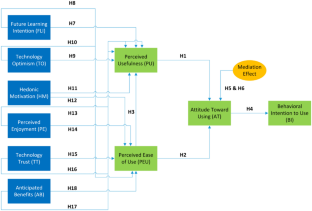
“Extending the Technology Acceptance Model (TAM) to Predict University Students’ Intentions to Use Metaverse-Based Learning Platforms”

Exploring the drivers of technology acceptance: a study of Nepali school students

A new integrated model to explore factors that influence adoption of mobile learning in higher education: An empirical investigation
Availability of data and materials.
The datasets generated and analysed during the current study are available from the corresponding author on reasonable request.
Kim J. Advertising in the metaverse: research agenda. J Interact Advert. 2021;21:141–4. https://doi.org/10.1080/15252019.2021.2001273 .
Article Google Scholar
Jeon JE. The effects of user experience-based design innovativeness on user– metaverse platform channel relationships in South Korea. J Distrib Sci. 2021;19:81–90. https://doi.org/10.15722/jds.19.11.202111.81 .
Lee SG, Trimi S, Byun WK, Kang M. Innovation and imitation effects in Metaverse service adoption. Serv Bus. 2011;5:155–72. https://doi.org/10.1007/s11628-011-0108-8 .
Siyaev A, Jo GS. Towards aircraft maintenance metaverse using speech interactions with virtual objects in mixed reality. Sensors. 2021;21:1–21. https://doi.org/10.3390/s21062066 .
Shen B, Tan W, Guo J, Zhao L, Qin P. How to promote user purchase in metaverse? A systematic literature review on consumer behavior research and virtual commerce application design. Appl Sci. 2021. https://doi.org/10.3390/app112311087 .
Koo S. An observation on possibility for applying metaverse concept to passenger car instrument panel design. Trans KSAE. 2021;29:1041–51.
Park S, Kim SP, Whang M. Individual’s social perception of virtual avatars embodied with their habitual facial expressions and facial appearance. Sensors. 2021. https://doi.org/10.3390/s21175986 .
Díaz JEM, Saldaña CAD, Avila CAR. Virtual world as a resource for hybrid education. Int J Emerg Technol Learn. 2020;15:94–109. https://doi.org/10.3991/ijet.v15i15.13025 .
Han J, Heo J, You E. Analysis of Metaverse Platform as a New Play Culture: Focusing on Roblox and ZEPETO. In: Nam D. Vo, O-Joun Lee, Khac-Hoai Nam Bui, Hae Gyun Lim, Hyeon-Ju Jeon, Phuong-Mai Nguyen, et al., editors. Comput. 2021 2nd Int. Conf. Human-centered Artif. Intell. Da Nang, Vietnam: CEUR Workshop Proceedings; 2021.
Sardar A, Garaniya V, Anantharaman M, Abbassi R, Khan F. Comparison between simulation and conventional training: expanding the concept of social fidelity. Process Saf Prog. 2022;41:S27-38. https://doi.org/10.1002/prs.12361 .
De Medios R, Educación. Píxel-Bit. Revista de Medios y Educación PIXEL-BIT. Pixel Bit. 2021. pp. 10–1.
Looi KH. Overcoming challenges to make e-learning a panacea for present and future crises. Int J Inf Learn Technol. 2022;39:227–39. https://doi.org/10.1108/IJILT-10-2021-0157 .
Kamri KA, Isa K, Yahya A, Ahmad AR, Yusoff R. Factors influencing alumni donations at Malaysian public universities. Proc. 28th Int. Bus. Inf. Manag. Assoc. Conf. - Vis. 2020 Innov. Manag. Dev. Sustain. Compet. Econ. Growth. 2016. pp. 278–286.
Davis FD. Perceived usefulness, perceived ease of use, and user acceptance of information technology. MIS Q. 1989;13:319–40. https://doi.org/10.2307/249008 .
Rosli MS, Saleh NS. Technology enhanced learning acceptance among university students during Covid-19: Integrating the full spectrum of Self-Determination Theory and self-efficacy into the Technology Acceptance Model. Curr Psychol. 2023;42:18212–31. https://doi.org/10.1007/s12144-022-02996-1 .
Saari UA, Tossavainen A, Kaipainen K, Mäkinen SJ. Exploring factors influencing the acceptance of social robots among early adopters and mass market representatives. Rob Auton Syst. 2022;151: 104033. https://doi.org/10.1016/J.ROBOT.2022.104033 .
Liébana-Cabanillas F, Marinković V, Kalinić Z. A SEM-neural network approach for predicting antecedents of m-commerce acceptance. Int J Inf Manage. 2017;37:14–24. https://doi.org/10.1016/j.ijinfomgt.2016.10.008 .
Shang D, Wu W. Understanding mobile shopping consumers’ continuance intention. Ind Manag Data Syst. 2017;117:213–27. https://doi.org/10.1108/IMDS-02-2016-0052 .
Cao D, Tao H, Wang Y, Tarhini A, Xia S. Acceptance of automation manufacturing technology in China: an examination of perceived norm and organizational efficacy. Prod Plan Control. 2020;31:660–72. https://doi.org/10.1080/09537287.2019.1669091 .
Holden RJ, Karsh BT. The Technology Acceptance Model: Its past and its future in health care. J Biomed Inform. 2010;43:159–72. https://doi.org/10.1016/j.jbi.2009.07.002 .
Venkatesh V, Morris MG, Davis GB, Davis FD. User acceptance of information technology: toward a unified view. MIS Q. 2003;27:425–78. https://doi.org/10.2307/30036540 .
Šumak B, Heričko M, Pušnik M. A meta-analysis of e-learning technology acceptance: the role of user types and e-learning technology types. Comput Human Behav. 2011;27:2067–77. https://doi.org/10.1016/j.chb.2011.08.005 .
Granić A, Marangunić N. Technology acceptance model in educational context: a systematic literature review. Br J Educ Technol. 2019;50:2572–93. https://doi.org/10.1111/bjet.12864 .
Rosli MS, Saleh NS, Md. Ali A, Abu Bakar S, Mohd Tahir L. A Systematic Review of the Technology Acceptance Model for the Sustainability of Higher Education during the COVID-19 Pandemic and Identified Research Gaps. Sustainability. 2022; https://doi.org/10.3390/su141811389 .
Xue L, Rashid AM, Ouyang S. The Unified Theory of Acceptance and Use of Technology (UTAUT) in higher education: a systematic review. SAGE Open. 2024;14:1–22. https://doi.org/10.1177/21582440241229570 .
Taherdoost H. A review of technology acceptance and adoption models and theories. Procedia Manuf. 2018;22:960–7.
Nezamdoust S, Abdekhoda M, Rahmani A. Determinant factors in adopting mobile health application in healthcare by nurses. BMC Med Inform Decis Mak. 2022;22:47. https://doi.org/10.1186/s12911-022-01784-y .
Abdullah F, Ward R, Ahmed E. Investigating the influence of the most commonly used external variables of TAM on students’ Perceived Ease of Use (PEOU) and Perceived Usefulness (PU) of e-portfolios. Comput Human Behav. 2016;63:75–90. https://doi.org/10.1016/j.chb.2016.05.014 .
Turner M, Kitchenham B, Brereton P, Charters S, Budgen D. Does the technology acceptance model predict actual use? A systematic literature review. Inf Softw Technol. 2010;52:463–79. https://doi.org/10.1016/j.infsof.2009.11.005 .
Alhamad AQM, Akour I, Alshurideh M, Al-Hamad AQ, Kurdi B Al, Alzoubi H. Predicting the intention to use google glass: A comparative approach using machine learning models and PLS-SEM. Int J Data Netw Sci. 2021;5:311–20. https://doi.org/10.5267/j.ijdns.2021.6.002 .
Pelegrín-Borondo J, Reinares-Lara E, Olarte-Pascual C. Assessing the acceptance of technological implants (the cyborg): Evidences and challenges. Comput Human Behav. 2017;70:104–12. https://doi.org/10.1016/j.chb.2016.12.063 .
Oeldorf-Hirsch A, Chen Y. Mobile mindfulness: predictors of mobile screen time tracking. Comput Human Behav. 2022;129: 107170. https://doi.org/10.1016/j.chb.2021.107170 .
Mustofa RH, Pramudita DA, Atmono D, Priyankara R, Asmawan MC, Rahmattullah M, et al. Exploring educational students acceptance of using movies as economics learning media: PLS-SEM analysis. Int Rev Econ Educ. 2022;39: 100236. https://doi.org/10.1016/J.IREE.2022.100236 .
Scherer R, Teo T. Editorial to the special section—Technology acceptance models: What we know and what we (still) do not know. Br J Educ Technol. 2019;50:2387–93. https://doi.org/10.1111/bjet.12866 .
Huang T. Using SOR framework to explore the driving factors of older adults smartphone use behavior. Humanit Soc Sci Commun. 2023;10:690. https://doi.org/10.1057/s41599-023-02221-9 .
Lavidas K, Komis V, Achriani A. Explaining faculty members’ behavioral intention to use learning management systems. J Comput Educ. 2022;9:707–25. https://doi.org/10.1007/s40692-021-00217-5 .
Gurer MD. Examining technology acceptance of pre-service mathematics teachers in Turkey: a structural equation modeling approach. Educ Inf Technol. 2021;26:4709–29. https://doi.org/10.1007/s10639-021-10493-4 .
Ho JC, Wu C-G, Lee C-S, Pham T-TT. Factors affecting the behavioral intention to adopt mobile banking: an international comparison. Technol Soc. 2020;63:101360. https://doi.org/10.1016/j.techsoc.2020.101360 .
Moon H, Hong S. The multiple mediating effects of Korean workers’ perception of the fourth industrial revolution, career attitudes and future learning intent. Eur J Train Dev. 2022. https://doi.org/10.1108/EJTD-06-2021-0073 .
Ng C. Australian primary students’ motivation and learning intentions for extra-curricular music programmes. Music Educ Res. 2017;19:276–91. https://doi.org/10.1080/14613808.2015.1095721 .
Lo Presti A, De Rosa A, Viceconte E. I want to learn more! Integrating technology acceptance and task–technology fit models for predicting behavioural and future learning intentions. J Work Learn. 2021;33:591–605. https://doi.org/10.1108/JWL-11-2020-0179 .
Liu Y, Gan Y, Song Y, Liu J. What influences the perceived trust of a voice-enabled smart home system: an empirical study. Sensors. 2021;21:1–22. https://doi.org/10.3390/s21062037 .
Shin HH, Jeong M. Redefining luxury service with technology implementation: the impact of technology on guest satisfaction and loyalty in a luxury hotel. Int J Contemp Hosp Manag. 2022;34:1491–514. https://doi.org/10.1108/IJCHM-06-2021-0798 .
Álvarez-Marín A, Velázquez-Iturbide JÁ, Castillo-Vergara M. Technology acceptance of an interactive augmented reality app on resistive circuits for engineering students. Electron. 2021. https://doi.org/10.3390/electronics10111286 .
Venkatesh V, Thong JYL, Xu X. Consumer acceptance and use of information technology: extending the unified theory of acceptance and use of technology. MIS Q. 2012;36:157–78. https://doi.org/10.2307/41410412 .
Kim KJ. Round or square? How screen shape affects utilitarian and hedonic motivations for smartwatch adoption. Cyberpsychol Behav Soc Netw. 2016;19:733–9. https://doi.org/10.1089/cyber.2016.0136 .
Kala Kamdjoug JR, Wamba-Taguimdje SL, Wamba SF, Kake IB e. Determining factors and impacts of the intention to adopt mobile banking app in Cameroon: Case of SARA by afriland First Bank. J Retail Consum Serv. 2021;61:102509. https://doi.org/10.1016/J.JRETCONSER.2021.102509 .
Abdul Rabu SN, Hussin H, Bervell B. QR code utilization in a large classroom: Higher education students’ initial perceptions. Educ Inf Technol. 2019;24:359–84. https://doi.org/10.1007/s10639-018-9779-2 .
Salimon MG, Aliyu OA, Yusr MM, Perumal S. Smartphone banking usage in Nigeria: Gamification, technology acceptance and cultural factors empirical perspectives. Electron J Inf Syst Dev Ctries. 2021;87: e12174. https://doi.org/10.1002/isd2.12174 .
Moghavvemi S, Paramanathan T, Rahin NM, Sharabati M. Student’s perceptions towards using e-learning via Facebook. Behav Inf Technol. 2017;36:1081–100. https://doi.org/10.1080/0144929X.2017.1347201 .
Kumar JA, Bervell B. Google Classroom for mobile learning in higher education: Modelling the initial perceptions of students. Educ Inf Technol. 2019;24:1793–817. https://doi.org/10.1007/s10639-018-09858-z .
Davis FD, Bagozzi RP, Warshaw PR. Extrinsic and intrinsic motivation to use computers in the workplace. J Appl Soc Psychol. 1992;22:1111–32. https://doi.org/10.1111/j.1559-1816.1992.tb00945.x .
Johar SS. The impact of emotional intelligence competencies on self-esteem among public servants. Indian J Public Heal Res Dev. 2019;10:1598–603. https://doi.org/10.5958/0976-5506.2019.01524.9 .
Lee CBP, Wan G. Including subjective norm and technology trust in the technology acceptance model: a case of e-ticketing in China. Data Base Adv Inf Syst. 2010;41:40–51. https://doi.org/10.1145/1899639.1899642 .
Sarfraz M, Khawaja KF, Ivascu L. Factors affecting business school students’ performance during the COVID-19 pandemic: a moderated and mediated model. Int J Manag Educ. 2022;20: 100630. https://doi.org/10.1016/j.ijme.2022.100630 .
Al Shamsi JH, Al-Emran M, Shaalan K. Understanding key drivers affecting students’ use of artificial intelligence-based voice assistants. Educ Inf Technol. 2022. https://doi.org/10.1007/S10639-022-10947-3 .
Venters W, Whitley EA. A critical review of cloud computing: researching desires and realities. J Inf Technol. 2012;27:179–97. https://doi.org/10.1057/jit.2012.17 .
Ali O, Shrestha A, Osmanaj V, Muhammed S. Cloud computing technology adoption: an evaluation of key factors in local governments. Inf Technol People. 2021;34:666–703. https://doi.org/10.1108/ITP-03-2019-0119 .
Albayati H. Investigating undergraduate students’ perceptions and awareness of using ChatGPT as a regular assistance tool: A user acceptance perspective study. Comput Educ Artif Intell. 2024;6:100203. https://doi.org/10.1016/j.caeai.2024.100203 .
Teo T, Milutinovic V. Modelling the intention to use technology for teaching mathematics among pre-service teachers in Serbia. Australas J Educ Technol. 2015; https://doi.org/10.14742/ajet.1668 .
Hair J, Black W, Babin B, Anderson R. Multivariate data analysis: a global perspective. Multivar. Data Anal. A Glob. Perspect., vol. 7th. New Jersey: Pearson Education; 2010.
Wolf EJ, Harrington KM, Clark SL, Miller MW. Sample size requirements for structural equation models: an evaluation of power, bias, and solution propriety. Educ Psychol Meas. 2013;73:913–34. https://doi.org/10.1177/0013164413495237 .
Yıldız O. PLS-SEM bias: traditional vs consistent. Qual Quant. 2023;57:537–52. https://doi.org/10.1007/s11135-021-01289-2 .
Rosseel Y. Small sample solutions for structural equation modeling. Small sample size Solut. Routledge; 2020. pp. 226–38.
De Jonckere J, Rosseel Y. Using bounded estimation to avoid nonconvergence in small sample structural equation modeling. Struct Equ Model A Multidiscip J. 2022;29:412–27. https://doi.org/10.1080/10705511.2021.1982716 .
Article MathSciNet Google Scholar
de Andrés-Sánchez J, Gené-Albesa J. Not with the bot! The relevance of trust to explain the acceptance of chatbots by insurance customers. Humanit Soc Sci Commun. 2024;11:110. https://doi.org/10.1057/s41599-024-02621-5 .
Sun PP, Luo X. Understanding English-as-a-foreign-language university teachers’ synchronous online teaching satisfaction: a Chinese perspective. J Comput Assist Learn. 2024;40:685–96. https://doi.org/10.1111/jcal.12891 .
Farooq A, Warkentin M, Virtanen S. Role of shared identity and agency trust in online voting among Finnish citizens. Technol Soc. 2024;76:102429. https://doi.org/10.1016/j.techsoc.2023.102429 .
Vijh G, Sharma R, Agrawal S. Blockchain-enabled intelligent solution using structured equation modelling based on the UTAUT framework. SN Comput Sci. 2023;4:738. https://doi.org/10.1007/s42979-023-02150-z .
Saif N, Khan SU, Shaheen I, ALotaibi A, Alnfiai MM, Arif M. Chat-GPT; validating Technology Acceptance Model (TAM) in education sector via ubiquitous learning mechanism. Comput Human Behav. 2024;154:108097. https://doi.org/10.1016/j.chb.2023.108097 .
Fornell C, Larcker DDF. Evaluating structural equation models with unobservable variables and measurement error. J Mark Res. 1981;18:39–50. https://doi.org/10.2307/3151312 .
Hu LT, Bentler PM. Cutoff criteria for fit indexes in covariance structure analysis: Conventional criteria versus new alternatives. 1999;6:1–55. https://doi.org/10.1080/10705519909540118
Huang F, Teo T, Zhou M. Chinese students’ intentions to use the Internet-based technology for learning. Educ Technol Res Dev. 2020;68:575–91. https://doi.org/10.1007/s11423-019-09695-y .
Sivo SA, Ku CH, Acharya P. Understanding how university student perceptions of resources affect technology acceptance in online learning courses. Australas J Educ Technol. 2018;34:72–91. https://doi.org/10.14742/ajet.2806 .
Wang X, Goh DHL, Lim EP. Understanding continuance intention toward crowdsourcing games: a longitudinal investigation. Int J Hum Comput Interact. 2020;36:1168–77. https://doi.org/10.1080/10447318.2020.1724010 .
Al-Maroof RS, Akour I, Aljanada R, Alfaisal AM, Alfaisal RM, Aburayya A, et al. Acceptance determinants of 5G services. Int J Data Netw Sci. 2021;5:613–28. https://doi.org/10.5267/j.ijdns.2021.8.006 .
Almarashdeh I, Eldaw KE, Alsmadi M, Alghamdi F, Jaradat G, Althunibat A, et al. The adoption of bitcoins technology: The difference between perceived future expectation and intention to use bitcoins: Does social influence matter? Int J Electr Comput Eng. 2021;11:5351–66. https://doi.org/10.11591/ijece.v11i6.pp5351-5366 .
Byrne BM. Structural equation modeling with AMOS : basic concepts, applications, and programming. Third Edit: Routledge; 2016.
Book Google Scholar
Hair JF, Risher JJ, Sarstedt M, Ringle CM. When to use and how to report the results of PLS-SEM. Eur Bus Rev. 2019;31:2–24. https://doi.org/10.1108/EBR-11-2018-0203 .
Gaskin J, Lim J. Model fit measures, AMOS plugin. Gaskination’s StatWiki. 2016;1–55.
Henseler J, Ringle CM, Sarstedt M. A new criterion for assessing discriminant validity in variance-based structural equation modeling. J Acad Mark Sci. 2015;43:115–35. https://doi.org/10.1007/s11747-014-0403-8 .
Gaskin J, Godfrey S, Vance A. Successful System-use: It’s Not Just Who You Are, But What You Do. AIS Trans Human-Computer Interact. 2018;10:57–81. https://doi.org/10.17705/1thci.00104 .
Cárdenas-Sainz BA, Barrón-Estrada ML, Zatarain-Cabada R, Ríos-Félix JM. Integration and acceptance of Natural User Interfaces for interactive learning environments. Int J Child-Computer Interact. 2022;31: 100381. https://doi.org/10.1016/j.ijcci.2021.100381 .
Bag S, Aich P, Islam MA. Behavioral intention of “digital natives” toward adapting the online education system in higher education. J Appl Res High Educ. 2022;14:16–40. https://doi.org/10.1108/JARHE-08-2020-0278 .
Hsu CL, Lin JCC. Acceptance of blog usage: The roles of technology acceptance, social influence and knowledge sharing motivation. Inf Manag. 2008;45:65–74. https://doi.org/10.1016/j.im.2007.11.001 .
Humida T, Al Mamun MH, Keikhosrokiani P. Predicting behavioral intention to use e-learning system: a case-study in Begum Rokeya University, Rangpur, Bangladesh. Educ Inf Technol. 2022;27:2241–65. https://doi.org/10.1007/s10639-021-10707-9 .
Perry A. Consumers’ acceptance of smart virtual closets. J Retail Consum Serv. 2016;33:171–7. https://doi.org/10.1016/j.jretconser.2016.08.018 .
Kowalczuk P. Consumer acceptance of smart speakers: a mixed methods approach. J Res Interact Mark. 2018;12:418–31. https://doi.org/10.1108/JRIM-01-2018-0022 .
Álvarez-Marín A, Velázquez-Iturbide JÁ, Castillo-Vergara M. The acceptance of augmented reality in engineering education: the role of technology optimism and technology innovativeness. Interact Learn Environ. 2021;0:1–13. https://doi.org/10.1080/10494820.2021.1928710 .
Chao CM, Yu TK. The moderating effect of technology optimism: How it affects students’ weblog learning. Online Inf Rev. 2019;43:161–80. https://doi.org/10.1108/OIR-11-2016-0316 .
Abdullah F, Ward R. Developing a General Extended Technology Acceptance Model for E-Learning (GETAMEL) by analysing commonly used external factors. Comput Human Behav. 2016;56:238–56. https://doi.org/10.1016/j.chb.2015.11.036 .
Li W, Shen S, Yang J, Tang Q. Internet-based medical service use and eudaimonic well-being of urban older adults: a peer support and technology acceptance model. Int J Environ Res Public Health. 2021. https://doi.org/10.3390/ijerph182212062 .
Daher W, Baya’a N, Anabousy A. Emotions and self-efficacy as mediators of pre-service teachers’ adoption of digital tools. Emerg Sci J. 2021;5:636–49. https://doi.org/10.28991/esj-2021-01301 .
Pouli V, Kafetzoglou S, Tsiropoulou EE, Dimitriou A, Papavassiliou S. Personalized multimedia content retrieval through relevance feedback techniques for enhanced user experience. 2015 13th Int. Conf. Telecommun. 2015. pp. 1–8. https://doi.org/10.1109/ConTEL.2015.7231205 .
Download references
The authors declare that no funds, grants, or other support were received during the preparation of this manuscript.
Author information
Authors and affiliations.
School of Education, Faculty of Social Sciences and Humanities, Universiti Teknologi Malaysia, 81310, Johor Bahru, Malaysia
Mohd Shafie Rosli
Department of Social Science, Centre for General Studies and Co-Curricular, Universiti Tun Hussein Onn Malaysia, 86400, Batu Pahat, Malaysia
Nor Shela Saleh
You can also search for this author in PubMed Google Scholar
Contributions
Conceptualization: Mohd Shafie Rosli; Methodology: Nor Shela Saleh; Formal analysis and investigation: Mohd Shafie Rosli, Nor Shela Saleh; Writing – original draft preparation: Mohd Shafie Rosli; Writing – review and editing: Nor Shela Saleh.
Corresponding author
Correspondence to Mohd Shafie Rosli .
Ethics declarations
Conflict of interest.
The authors have no relevant financial or non-financial interests to disclose.
Ethical Approval
All the data collection procedures were in accordance with the ethical practices. Ethical approval was not required in accordance with the current institutional requirement where the data were collected.
Informed Consent
Respondents answered the questionnaire voluntarily and were informed about the research purposes before they agreed to answer the questionnaire.
Additional information
Publisher's note.
Springer Nature remains neutral with regard to jurisdictional claims in published maps and institutional affiliations.
Rights and permissions
Springer Nature or its licensor (e.g. a society or other partner) holds exclusive rights to this article under a publishing agreement with the author(s) or other rightsholder(s); author self-archiving of the accepted manuscript version of this article is solely governed by the terms of such publishing agreement and applicable law.
Reprints and permissions
About this article
Rosli, M.S., Saleh, N.S. Predicting the Acceptance of Metaverse for Educational Purposes in Universities: A Structural Equation Model and Mediation Analysis of the Extended Technology Acceptance Model. SN COMPUT. SCI. 5 , 688 (2024). https://doi.org/10.1007/s42979-024-03015-9
Download citation
Received : 26 June 2023
Accepted : 30 May 2024
Published : 02 July 2024
DOI : https://doi.org/10.1007/s42979-024-03015-9
Share this article
Anyone you share the following link with will be able to read this content:
Sorry, a shareable link is not currently available for this article.
Provided by the Springer Nature SharedIt content-sharing initiative
- Technology acceptance model
- Structural equation model
- Find a journal
- Publish with us
- Track your research
IMAGES
VIDEO
COMMENTS
Abstract. Structural equation modeling is a multivariate data analysis method for analyzing complex relationships among constructs and indicators. To estimate structural equation models, researchers generally draw on two methods: covariance-based SEM (CB-SEM) and partial least squares SEM (PLS-SEM).
This literature review aimed to describe the use of structural equation modelling in research. In general, SEM can be used to analyze research models that have several independent (exogenous) and ...
Learning Objectives. After reading this chapter, you should: 1. Understand the principles of structural equation modeling (SEM) 2. Describe the basic elements of a structural equation model. 3. Comprehend the basic concepts of partial least squares structural equation modeling (PLS-SEM) 4.
This is exactly where SEM comes in. SEM can assist L2 researchers to model and assess more complex relationships of multiple variables, manifest or latent, in a single study. SEM use gained in popularity by the development of a computer program to examine linear structural relationships (LISREL) by Jöreskog (1970).
This review was developed to introduce the essential components and variants of structural equation modeling (SEM), synthesize the common issues in SEM applications, and share our views on SEM's future in ecological research. We searched the Web of Science on SEM applications in ecological studies from 1999 through 2016 and summarized the potential of SEMs, with a special focus on unexplored ...
for estimating θ, where Σ(θ) is the structural model.Unlike in linear regression where there is an analytical formula for estimating the regression coefficients, we have to use an iterative procedure to minimize F ml (θ), and the Fisher-scoring algorithm (see Lee and Jennrich, 1979) is typically used for such a purpose.Small N or large p can cause various problems when minimizing F ml (θ ...
1. Introduction. Since Bentler's appeal to apply the technique to handle latent variables (i.e. unobserved variables) in psychological science [8], structural equation modeling (SEM) has become a quasi-routine and even indispensable statistical analysis approach in the social sciences.Computer programs designed for conducting SEM analyses have emerged and enabled the technique to be used in ...
This paper is a tribute to researchers who have significantly contributed to improving and advancing structural equation modeling (SEM). It is, therefore, a brief overview of SEM and presents its beginnings, historical development, its usefulness in the social sciences and the statistical and philosophical (theoretical) controversies which have often appeared in the literature pertaining to ...
The structural equation modelling (SEM) method has stronger predicting power than path analysis and multiple regression because SEM is able to analyze at the deepest level the variables or constructs studied. This literature review aimed to describe the use of structural equation modelling in research. In general, SEM can be used to analyze research models that have several independent ...
past literature and the Structural Equation Model (SEM) is one of the common techniques that has been used (Ismael and Duleba, 2021). The main aim of this article is to sys-tematically review the application of Structural Equation Modelling (SEM) approaches in the area of transporta-tion planning and sustainable transportation. An addi-
Abstract - The paper addresses an introduction to the structural equation modeling (SEM), the insight into the methodology, and the importance of this statistical technique for practical applications.
Structural equation models (SEMs) are a flexible class of. covariate effects on the exposure as well as their effect on the outcome. In Section 2 we discuss motivating examples and introduce. models that allow complex modeling of multivariate data and. multiple, closely related predictors.
The use of structural equation modeling (SEM) has grown substantially over the past 40 years within organizational research and beyond. There have been many different developments in SEM that make it increasingly useful for a variety of data types, research designs, research questions, and research contexts in the organizational sciences. To give researchers a better understanding of how and ...
We provide a comprehensive and user-friendly compendium of standards for the use and interpretation of structural equation models (SEMs). To both read about and do research that employs SEMs, it is necessary to master the art and science of the statistical procedures underpinning SEMs in an integrative way with the substantive concepts, theories, and hypotheses that researchers desire to examine.
However, there is still a gap in the literature regarding review papers in the field of environmental sustainability and Structural Equation Modelling (SEM).Therefore, the aim of this work is to conduct a systematic literature review of the application of SEM in examining environmental sustainability.
Structural equation modelling showed that more use of avoidance and impulsivity and less use of cognitive reappraisal negatively affected sleep quality, which, in turn, was associated with the ...
gap in the literature. To close this gap, this paper-based on prior AR studies-provided an overview of theory- ... A systematic review of structural equation modeling in augmented reality applications (Vinh The Nguyen) 331 the technology must be utilized and a good fit with the tasks it supports to have positive impacts on individual ...
An increasing number of studies applying structural equation modelling have been witnessed to the research on teaching and teacher education. This paper reviews 15 of 132 articles that use structural equation modelling as the main strategy of data analysis published in Teaching and Teacher Education from 1985 to 2020. The 15 articles touch on three themes of teaching and teacher education ...
The use of various structural equation modelling methods in social work research con-tinues to expand. As more social work researchers become acquainted with structural equation modelling (SEM), there has been an increase in the application of the methods in social work academic journals. The study reported here is a systematic review of the lit-
Conceptual model and hypothesis development. In this paper, a conceptual model has been developed through an examination of scientific literature (Fig 1) and tested through partial least square structural equation modelling.The purpose of model is to address the needs smallholders by organizing value chain actors, and what factors should be considered to reduce transaction cost and manage ...
Structural equation modeling (SEM) is a comprehensive statistical approach to testing hypotheses about relations among observed and latent variables (Hoyle, 1995). is a methodology for representing, estimating, and testing a theoretical network of (mostly) linear relations between variables (Rigdon, 1998).
This study aims to evaluate the usage of partial least squares structural equation modeling (PLS-SEM) in journals related to logistics and supply chain management (LSCM).,Based on a structured literature review approach, the authors reviewed 401 articles in the field of LSCM applying PLS-SEM published in 15 major journals between 2014 and 2022.
Ohta, M. et al. Structural equation modeling approach between salience network dysfunction, depressed mood, and subjective quality of life in schizophrenia: An ICA resting-state fMRI study ...
For this, we first show how DAGs for measurement models can be translated into path diagrams used in the linear structural equation model (SEM) literature. We then demonstrate how insights gained from this causal perspective can be used to explicitly model encoded causal assumptions with moderated SEMs, allowing for a more enlightening ...
This research on electric vehicle purchasing intentions in Thailand using Structural Equation Modeling aimed to achieve the following objectives: Firstly, to investigate the factors influencing consumers' intentions to purchase electric vehicles. Secondly, to examine the impact of consumer characteristics on supply chain agility (SCA). Thirdly, to analyze how electric vehicle characteristics ...
Structural equation modeling (SEM) is a very powerful multivariate statistical technique that has increasingly been used in social sciences, particularly in marketing. ... Critical Review of the ...
With the emerging large- and medium-sized engineering projects, prominent project delivery methods make sense in terms of cost, risk, management, and schedule. Among these, the Integrated Project Delivery (IPD) method stands out due to its adaptability for growing scale and complexity projects. This study compares the IPD method with other methods, emphasizing its benefits in large- and medium ...
The technique of meta-analytic structural equation modeling (MASEM) was applied to analyze the aggregated data. Moderator analyses examined the role of individual characteristics in the relations between (1) mindfulness and decentering, (2) decentering and psychological problems, and (3) mindfulness and psychological problems.
For examining the structural relationships, we have used covariance-based structural equation modelling (SEM). We have found that contextual factors like brand perception of investment, economic fundamentals, and individual financial needs are positively associated with investor sentiments. ... Global Business and Economics Review, 2024 Vol.31 ...
The extended Technology Acceptance Model consists of 18 hypotheses that were tested using the Structural Equation Model and Mediation Analysis with data from 215 university students. ... A recent systematic literature review of the Technology Acceptance Model by Rosli et al. employing the PRISMA statement and guideline revealed that Self ...