assignments k means

K-Means Clustering

3 assignment k-means clustering.

Let’s apply K-means clustering on the same data set we used for kNN.

You have to determine a number of still unknown clusters of, in this case, makes and models of cars.

There is no criterion that we can use as a training and test set!

The questions and assignments are:

Read the file ( cars.csv ).
You have seen from the description in the previous assignment that the variable for origin (US, versus non-US) is a factor variable. We cannot calculate distances from a factor variable. Because we want to include it anyway, we have to make it a dummy (0/1) variable.
Normalize the data.
Determine the number of clusters using the (graphical) method described above.
Determine the clustering, and add the cluster to the data set.
Describe the clusters in terms of all variables used in the clustering.
Characterize ( label ) the clusters.
Repeat the exercise with more or fewer clusters, and decide if the new solutions are better than the original solution!

3.1 Solution: Some Help

Read the data:

And make a function for normalizing your data:

And normalize the data, after creating a dummy for origin .

The normalized data to use, are now in cars2_n .

Decide on the best number of clusters:

The text is released under the CC-BY-NC-ND license , and code is released under the MIT license . If you find this content useful, please consider supporting the work by buying the book !

In Depth: k-Means Clustering

< In-Depth: Manifold Learning | Contents | In Depth: Gaussian Mixture Models >

In the previous few sections, we have explored one category of unsupervised machine learning models: dimensionality reduction. Here we will move on to another class of unsupervised machine learning models: clustering algorithms. Clustering algorithms seek to learn, from the properties of the data, an optimal division or discrete labeling of groups of points.

Many clustering algorithms are available in Scikit-Learn and elsewhere, but perhaps the simplest to understand is an algorithm known as k-means clustering , which is implemented in sklearn.cluster.KMeans .

We begin with the standard imports:

Introducing k-Means ¶

The k -means algorithm searches for a pre-determined number of clusters within an unlabeled multidimensional dataset. It accomplishes this using a simple conception of what the optimal clustering looks like:

The "cluster center" is the arithmetic mean of all the points belonging to the cluster.
Each point is closer to its own cluster center than to other cluster centers.

Those two assumptions are the basis of the k -means model. We will soon dive into exactly how the algorithm reaches this solution, but for now let's take a look at a simple dataset and see the k -means result.

First, let's generate a two-dimensional dataset containing four distinct blobs. To emphasize that this is an unsupervised algorithm, we will leave the labels out of the visualization

By eye, it is relatively easy to pick out the four clusters. The k -means algorithm does this automatically, and in Scikit-Learn uses the typical estimator API:

Let's visualize the results by plotting the data colored by these labels. We will also plot the cluster centers as determined by the k -means estimator:

The good news is that the k -means algorithm (at least in this simple case) assigns the points to clusters very similarly to how we might assign them by eye. But you might wonder how this algorithm finds these clusters so quickly! After all, the number of possible combinations of cluster assignments is exponential in the number of data points—an exhaustive search would be very, very costly. Fortunately for us, such an exhaustive search is not necessary: instead, the typical approach to k -means involves an intuitive iterative approach known as expectation–maximization .

k-Means Algorithm: Expectation–Maximization ¶

Expectation–maximization (E–M) is a powerful algorithm that comes up in a variety of contexts within data science. k -means is a particularly simple and easy-to-understand application of the algorithm, and we will walk through it briefly here. In short, the expectation–maximization approach here consists of the following procedure:

Guess some cluster centers
E-Step : assign points to the nearest cluster center
M-Step : set the cluster centers to the mean

Here the "E-step" or "Expectation step" is so-named because it involves updating our expectation of which cluster each point belongs to. The "M-step" or "Maximization step" is so-named because it involves maximizing some fitness function that defines the location of the cluster centers—in this case, that maximization is accomplished by taking a simple mean of the data in each cluster.

The literature about this algorithm is vast, but can be summarized as follows: under typical circumstances, each repetition of the E-step and M-step will always result in a better estimate of the cluster characteristics.

We can visualize the algorithm as shown in the following figure. For the particular initialization shown here, the clusters converge in just three iterations. For an interactive version of this figure, refer to the code in the Appendix .

(run code in Appendix to generate image)

The k -Means algorithm is simple enough that we can write it in a few lines of code. The following is a very basic implementation:

Most well-tested implementations will do a bit more than this under the hood, but the preceding function gives the gist of the expectation–maximization approach.

Caveats of expectation–maximization ¶

There are a few issues to be aware of when using the expectation–maximization algorithm.

The globally optimal result may not be achieved ¶

First, although the E–M procedure is guaranteed to improve the result in each step, there is no assurance that it will lead to the global best solution. For example, if we use a different random seed in our simple procedure, the particular starting guesses lead to poor results:

Here the E–M approach has converged, but has not converged to a globally optimal configuration. For this reason, it is common for the algorithm to be run for multiple starting guesses, as indeed Scikit-Learn does by default (set by the n_init parameter, which defaults to 10).

The number of clusters must be selected beforehand ¶

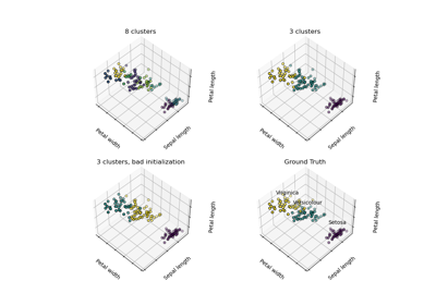
Another common challenge with k -means is that you must tell it how many clusters you expect: it cannot learn the number of clusters from the data. For example, if we ask the algorithm to identify six clusters, it will happily proceed and find the best six clusters:

Whether the result is meaningful is a question that is difficult to answer definitively; one approach that is rather intuitive, but that we won't discuss further here, is called silhouette analysis .

Alternatively, you might use a more complicated clustering algorithm which has a better quantitative measure of the fitness per number of clusters (e.g., Gaussian mixture models; see In Depth: Gaussian Mixture Models ) or which can choose a suitable number of clusters (e.g., DBSCAN, mean-shift, or affinity propagation, all available in the sklearn.cluster submodule)

k-means is limited to linear cluster boundaries ¶

The fundamental model assumptions of k -means (points will be closer to their own cluster center than to others) means that the algorithm will often be ineffective if the clusters have complicated geometries.

In particular, the boundaries between k -means clusters will always be linear, which means that it will fail for more complicated boundaries. Consider the following data, along with the cluster labels found by the typical k -means approach:

This situation is reminiscent of the discussion in In-Depth: Support Vector Machines , where we used a kernel transformation to project the data into a higher dimension where a linear separation is possible. We might imagine using the same trick to allow k -means to discover non-linear boundaries.

One version of this kernelized k -means is implemented in Scikit-Learn within the SpectralClustering estimator. It uses the graph of nearest neighbors to compute a higher-dimensional representation of the data, and then assigns labels using a k -means algorithm:

We see that with this kernel transform approach, the kernelized k -means is able to find the more complicated nonlinear boundaries between clusters.

k-means can be slow for large numbers of samples ¶

Because each iteration of k -means must access every point in the dataset, the algorithm can be relatively slow as the number of samples grows. You might wonder if this requirement to use all data at each iteration can be relaxed; for example, you might just use a subset of the data to update the cluster centers at each step. This is the idea behind batch-based k -means algorithms, one form of which is implemented in sklearn.cluster.MiniBatchKMeans . The interface for this is the same as for standard KMeans ; we will see an example of its use as we continue our discussion.

Examples ¶

Being careful about these limitations of the algorithm, we can use k -means to our advantage in a wide variety of situations. We'll now take a look at a couple examples.

Example 1: k-means on digits ¶

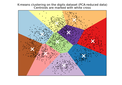
To start, let's take a look at applying k -means on the same simple digits data that we saw in In-Depth: Decision Trees and Random Forests and In Depth: Principal Component Analysis . Here we will attempt to use k -means to try to identify similar digits without using the original label information ; this might be similar to a first step in extracting meaning from a new dataset about which you don't have any a priori label information.

We will start by loading the digits and then finding the KMeans clusters. Recall that the digits consist of 1,797 samples with 64 features, where each of the 64 features is the brightness of one pixel in an 8×8 image:

The clustering can be performed as we did before:

The result is 10 clusters in 64 dimensions. Notice that the cluster centers themselves are 64-dimensional points, and can themselves be interpreted as the "typical" digit within the cluster. Let's see what these cluster centers look like:

We see that even without the labels , KMeans is able to find clusters whose centers are recognizable digits, with perhaps the exception of 1 and 8.

Because k -means knows nothing about the identity of the cluster, the 0–9 labels may be permuted. We can fix this by matching each learned cluster label with the true labels found in them:

Now we can check how accurate our unsupervised clustering was in finding similar digits within the data:

With just a simple k -means algorithm, we discovered the correct grouping for 80% of the input digits! Let's check the confusion matrix for this:

As we might expect from the cluster centers we visualized before, the main point of confusion is between the eights and ones. But this still shows that using k -means, we can essentially build a digit classifier without reference to any known labels !

Just for fun, let's try to push this even farther. We can use the t-distributed stochastic neighbor embedding (t-SNE) algorithm (mentioned in In-Depth: Manifold Learning ) to pre-process the data before performing k -means. t-SNE is a nonlinear embedding algorithm that is particularly adept at preserving points within clusters. Let's see how it does:

That's nearly 92% classification accuracy without using the labels . This is the power of unsupervised learning when used carefully: it can extract information from the dataset that it might be difficult to do by hand or by eye.

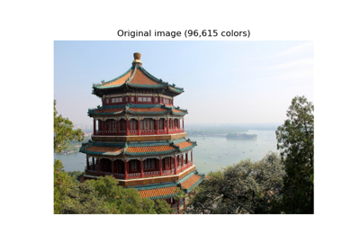
Example 2: k -means for color compression ¶

One interesting application of clustering is in color compression within images. For example, imagine you have an image with millions of colors. In most images, a large number of the colors will be unused, and many of the pixels in the image will have similar or even identical colors.

For example, consider the image shown in the following figure, which is from the Scikit-Learn datasets module (for this to work, you'll have to have the pillow Python package installed).

The image itself is stored in a three-dimensional array of size (height, width, RGB) , containing red/blue/green contributions as integers from 0 to 255:

One way we can view this set of pixels is as a cloud of points in a three-dimensional color space. We will reshape the data to [n_samples x n_features] , and rescale the colors so that they lie between 0 and 1:

We can visualize these pixels in this color space, using a subset of 10,000 pixels for efficiency:

Now let's reduce these 16 million colors to just 16 colors, using a k -means clustering across the pixel space. Because we are dealing with a very large dataset, we will use the mini batch k -means, which operates on subsets of the data to compute the result much more quickly than the standard k -means algorithm:

Definitive Guide to K-Means Clustering with Scikit-Learn

Introduction

K-Means clustering is one of the most widely used unsupervised machine learning algorithms that form clusters of data based on the similarity between data instances.

In this guide, we will first take a look at a simple example to understand how the K-Means algorithm works before implementing it using Scikit-Learn. Then, we'll discuss how to determine the number of clusters (Ks) in K-Means, and also cover distance metrics, variance, and K-Means pros and cons.

Imagine the following situation. One day, when walking around the neighborhood, you noticed there were 10 convenience stores and started to wonder which stores were similar - closer to each other in proximity. While searching for ways to answer that question, you've come across an interesting approach that divides the stores into groups based on their coordinates on a map.

For instance, if one store was located 5 km West and 3 km North - you'd assign (5, 3) coordinates to it, and represent it in a graph. Let's plot this first point to visualize what's happening:

This is just the first point, so we can get an idea of how we can represent a store. Say we already have 10 coordinates to the 10 stores collected. After organizing them in a numpy array, we can also plot their locations:

How to Manually Implement K-Means Algorithm

Now we can look at the 10 stores on a graph, and the main problem is to find is there a way they could be divided into different groups based on proximity? Just by taking a quick look at the graph, we'll probably notice two groups of stores - one is the lower points to the bottom-left, and the other one is the upper-right points. Perhaps, we can even differentiate those two points in the middle as a separate group - therefore creating three different groups .

In this section, we'll go over the process of manually clustering points - dividing them into the given number of groups. That way, we'll essentially carefully go over all steps of the K-Means clustering algorithm . By the end of this section, you'll gain both an intuitive and practical understanding of all steps performed during the K-Means clustering. After that, we'll delegate it to Scikit-Learn.

What would be the best way of determining if there are two or three groups of points? One simple way would be to simply choose one number of groups - for instance, two - and then try to group points based on that choice.

Let's say we have decided there are two groups of our stores (points). Now, we need to find a way to understand which points belong to which group. This could be done by choosing one point to represent group 1 and one to represent group 2 . Those points will be used as a reference when measuring the distance from all other points to each group.

In that manner, say point (5, 3) ends up belonging to group 1, and point (79, 60) to group 2. When trying to assign a new point (6, 3) to groups, we need to measure its distance to those two points. In the case of the point (6, 3) is closer to the (5, 3) , therefore it belongs to the group represented by that point - group 1 . This way, we can easily group all points into corresponding groups.

In this example, besides determining the number of groups ( clusters ) - we are also choosing some points to be a reference of distance for new points of each group.

That is the general idea to understand similarities between our stores. Let's put it into practice - we can first choose the two reference points at random . The reference point of group 1 will be (5, 3) and the reference point of group 2 will be (10, 15) . We can select both points of our numpy array by [0] and [1] indexes and store them in g1 (group 1) and g2 (group 2) variables:

After doing this, we need to calculate the distance from all other points to those reference points. This raises an important question - how to measure that distance. We can essentially use any distance measure, but, for the purpose of this guide, let's use Euclidean Distance_.

Advice: If you want learn more more about Euclidean distance, you can read our "Calculating Euclidean Distances with NumPy" guide.

It can be useful to know that Euclidean distance measure is based on Pythagoras' theorem:

$$ c^2 = a^2 + b^2 $$

When adapted to points in a plane - (a1, b1) and (a2, b2) , the previous formula becomes:

$$ c^2 = (a2-a1)^2 + (b2-b1)^2 $$

The distance will be the square root of c , so we can also write the formula as:

$$ euclidean_{dist} = \sqrt[2][(a2 - a1)^2 + (b2 - b1) ^2)] $$

Note: You can also generalize the Euclidean distance formula for multi-dimensional points. For example, in a three-dimensional space, points have three coordinates - our formula reflects that in the following way: $$ euclidean_{dist} = \sqrt[2][(a2 - a1)^2 + (b2 - b1) ^2 + (c2 - c1) ^2)] $$ The same principle is followed no matter the number of dimensions of the space we are operating in.

So far, we have picked the points to represent groups, and we know how to calculate distances. Now, let's put the distances and groups together by assigning each of our collected store points to a group.

To better visualize that, we will declare three lists. The first one to store points of the first group - points_in_g1 . The second one to store points from the group 2 - points_in_g2 , and the last one - group , to label the points as either 1 (belongs to group 1) or 2 (belongs to group 2):

We can now iterate through our points and calculate the Euclidean distance between them and each of our group references. Each point will be closer to one of two groups - based on which group is closest, we'll assign each point to the corresponding list, while also adding 1 or 2 to the group list:

Let's look at the results of this iteration to see what happened:

Which results in:

We can also plot the clustering result, with different colors based on the assigned groups, using Seaborn's scatterplot() with the group as a hue argument:

It's clearly visible that only our first point is assigned to group 1, and all other points were assigned to group 2. That result differs from what we had envisioned in the beginning. Considering the difference between our results and our initial expectations - is there a way we could change that? It seems there is!

One approach is to repeat the process and choose different points to be the references of the groups. This will change our results, hopefully, more in line with what we've envisioned in the beginning. This second time, we could choose them not at random as we previously did, but by getting a mean of all our already grouped points. That way, those new points could be positioned in the middle of corresponding groups.

For instance, if the second group had only points (10, 15) , (30, 45) . The new central point would be (10 + 30)/2 and (15+45)/2 - which is equal to (20, 30) .

Since we have put our results in lists, we can convert them first to numpy arrays, select their xs, ys and then obtain the mean :

Advice: Try to use numpy and NumPy arrays as much as possible. They are optimized for better performance and simplify many linear algebra operations. Whenever you are trying to solve some linear algebra problem, you should definitely take a look at the numpy documentation to check if there is any numpy method designed to solve your problem. The chance is that there is!

To help repeat the process with our new center points, let's transform our previous code into a function, execute it and see if there were any changes in how the points are grouped:

Note: If you notice you keep repeating the same code over and over again, you should wrap that code into a separate function. It is considered a best practice to organize code into functions, especially because they facilitate testing. It is easier to test an isolated piece of code than a full code without any functions.

Let's call the function and store its results in points_in_g1 , points_in_g2 , and group variables:

And also plot the scatter plot with the colored points to visualize the groups division:

It seems the clustering of our points is getting better . But still, there are two points in the middle of the graph that could be assigned to either group when considering their proximity to both groups. The algorithm we've developed so far assigns both of those points to the second group.

This means we can probably repeat the process once more by taking the means of the Xs and Ys, creating two new central points (centroids) to our groups and re-assigning them based on distance.

Let's also create a function to update the centroids. The whole process now can be reduced to multiple calls of that function:

Notice that after this third iteration, each one of the points now belong to different clusters. It seems the results are getting better - let's do it once again. Now going to the fourth iteration of our method:

This fourth time we got the same result as the previous one. So it seems our points won't change groups anymore, our result has reached some kind of stability - it has got to an unchangeable state, or converged . Besides that, we have exactly the same result as we had envisioned for the 2 groups. We can also see if this reached division makes sense.

Let's just quickly recap what we've done so far. We've divided our 10 stores geographically into two sections - ones in the lower southwest regions and others in the northeast. It can be interesting to gather more data besides what we already have - revenue, the daily number of customers, and many more. That way we can conduct a richer analysis and possibly generate more interesting results.

Clustering studies like this can be conducted when an already established brand wants to pick an area to open a new store. In that case, there are many more variables taken into consideration besides location.

What Does All This Have To Do With K-Means Algorithm?

While following these steps you might have wondered what they have to do with the K-Means algorithm. The process we've conducted so far is the K-Means algorithm . In short, we've determined the number of groups/clusters, randomly chosen initial points, and updated centroids in each iteration until clusters converged. We've basically performed the entire algorithm by hand - carefully conducting each step.

The K in K-Means comes from the number of clusters that need to be set prior to starting the iteration process. In our case K = 2 . This characteristic is sometimes seen as negative considering there are other clustering methods, such as Hierarchical Clustering, which don't need to have a fixed number of clusters beforehand.

Due to its use of means, K-means also becomes sensitive to outliers and extreme values - they enhance the variability and make it harder for our centroids to play their part. So, be conscious of the need to perform extreme values and outlier analysis before conducting a clustering using the K-Means algorithm.

Also, notice that our points were segmented in straight parts, there aren't curves when creating the clusters. That can also be a disadvantage of the K-Means algorithm.

Note: When you need it to be more flexible and adaptable to ellipses and other shapes, try using a generalized K-means Gaussian Mixture model . This model can adapt to elliptical segmentation clusters.

K-Means also has many advantages ! It performs well on large datasets which can become difficult to handle if you are using some types of hierarchical clustering algorithms. It also guarantees convergence , and can easily generalize and adapt . Besides that, it is probably the most used clustering algorithm.

Now that we've gone over all the steps performed in the K-Means algorithm, and understood all its pros and cons, we can finally implement K-Means using the Scikit-Learn library.

How to Implement K-Means Algorithm Using Scikit-Learn

To double check our result, let's do this process again, but now using 3 lines of code with sklearn :

Here, the labels are the same as our previous groups. Let's just quickly plot the result:

The resulting plot is the same as the one from the previous section.

Check out our hands-on, practical guide to learning Git, with best-practices, industry-accepted standards, and included cheat sheet. Stop Googling Git commands and actually learn it!

Note: Just looking at how we've performed the K-Means algorithm using Scikit-Learn might give you the impression that this is a no-brainer and that you don't need to worry too much about it. Just 3 lines of code perform all the steps we've discussed in the previous section when we've gone over the K-Means algorithm step-by-step. But, the devil is in the details in this case! If you don't understand all the steps and limitations of the algorithm, you'll most likely face the situation where the K-Means algorithm gives you results you were not expecting.

With Scikit-Learn, you can also initialize K-Means for faster convergence by setting the init='k-means++' argument. In broader terms, K-Means++ still chooses the k initial cluster centers at random following a uniform distribution. Then, each subsequent cluster center is chosen from the remaining data points not by calculating only a distance measure - but by using probability. Using the probability speeds up the algorithm and it's helpful when dealing with very large datasets.

Advice: You can learn more about K-Means++ details by reading the "K-Means++: The Advantages of Careful Seeding" paper, proposed in 2007 by David Arthur and Sergei Vassilvitskii.

The Elbow Method - Choosing the Best Number of Groups

So far, so good! We've clustered 10 stores based on the Euclidean distance between points and centroids. But what about those two points in the middle of the graph that are a little harder to cluster? Couldn't they form a separate group as well? Did we actually make a mistake by choosing K=2 groups? Maybe we actually had K=3 groups? We could even have more than three groups and not be aware of it.

The question being asked here is how to determine the number of groups (K) in K-Means . To answer that question, we need to understand if there would be a "better" cluster for a different value of K.

The naive way of finding that out is by clustering points with different values of K , so, for K=2, K=3, K=4, and so on :

But, clustering points for different Ks alone won't be enough to understand if we've chosen the ideal value for K . We need a way to evaluate the clustering quality for each K we've chosen.

Manually Calculating the Within Cluster Sum of Squares (WCSS)

Here is the ideal place to introduce a measure of how much our clustered points are close to each other. It essentially describes how much variance we have inside a single cluster. This measure is called Within Cluster Sum of Squares , or WCSS for short. The smaller the WCSS is, the closer our points are, therefore we have a more well-formed cluster. The WCSS formula can be used for any number of clusters:

$$ WCSS = \sum(Pi_1 - Centroid_1)^2 + \cdots + \sum(Pi_n - Centroid_n)^2 $$

Note: In this guide, we are using the Euclidean distance to obtain the centroids, but other distance measures, such as Manhattan, could also be used.

Now we can assume we've opted to have two clusters and try to implement the WCSS to understand better what the WCSS is and how to use it. As the formula states, we need to sum up the squared differences between all cluster points and centroids. So, if our first point from the first group is (5, 3) and our last centroid (after convergence) of the first group is (16.8, 17.0) , the WCSS will be:

$$ WCSS = \sum((5,3) - (16.8, 17.0))^2 $$

$$ WCSS = \sum((5-16.8) + (3-17.0))^2 $$

$$ WCSS = \sum((-11.8) + (-14.0))^2 $$

$$ WCSS = \sum((-25.8))^2 $$

$$ WCSS = 335.24 $$

This example illustrates how we calculate the WCSS for the one point from the cluster. But the cluster usually contains more than one point, and we need to take all of them into consideration when calculating the WCSS. We'll do that by defining a function that receives a cluster of points and centroids, and returns the sum of squares:

Now we can get the sum of squares for each cluster:

And sum up the results to obtain the total WCSS :

This results in:

So, in our case, when K is equal to 2, the total WCSS is 2964.39 . Now, we can switch Ks and calculate the WCSS for all of them. That way, we can get an insight into what K we should choose to make our clustering perform the best.

Calculating WCSS Using Scikit-Learn

Fortunately, we don't need to manually calculate the WCSS for each K . After performing the K-Means clustering for the given number of clusters, we can obtain its WCSS by using the inertia_ attribute. Now, we can go back to our K-Means for loop, use it to switch the number of clusters, and list corresponding WCSS values:

Notice that the second value in the list, is exactly the same we've calculated before for K=2 :

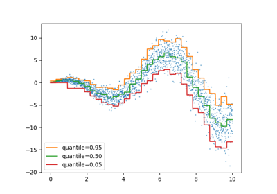
To visualize those results, let's plot our Ks along with the WCSS values:

There is an interruption on a plot when x = 2 , a low point in the line, and an even lower one when x = 3 . Notice that it reminds us of the shape of an elbow . By plotting the Ks along with the WCSS, we are using the Elbow Method to choose the number of Ks. And the chosen K is exactly the lowest elbow point , so, it would be 3 instead of 2 , in our case:

We can run the K-Means cluster algorithm again, to see how our data would look like with three clusters :

We were already happy with two clusters, but according to the elbow method, three clusters would be a better fit for our data. In this case, we would have three kinds of stores instead of two. Before using the elbow method, we thought about southwest and northeast clusters of stores, now we also have stores in the center. Maybe that could be a good location to open another store since it would have less competition nearby.

Alternative Cluster Quality Measures

There are also other measures that can be used when evaluating cluster quality:

Silhouette Score - analyzes not only the distance between intra-cluster points but also between clusters themselves
Between Clusters Sum of Squares (BCSS) - metric complementary to the WCSS
Sum of Squares Error (SSE)
Maximum Radius - measures the largest distance from a point to its centroid
Average Radius - the sum of the largest distance from a point to its centroid divided by the number of clusters.

It's recommended to experiment and get to know each of them since depending on the problem, some of the alternatives can be more applicable than the most widely used metrics (WCSS and Silhouette Score) .

In the end, as with many data science algorithms, we want to reduce the variance inside each cluster and maximize the variance between different clusters. So we have more defined and separable clusters.

Applying K-Means on Another Dataset

Let's use what we have learned on another dataset. This time, we will try to find groups of similar wines.

Note: You can download the dataset here .

We begin by importing pandas to read the wine-clustering CSV (Comma-Separated Values) file into a Dataframe structure:

After loading it, let's take a peek at the first five records of data with the head() method:

We have many measurements of substances present in wines. Here, we also won't need to transform categorical columns because all of them are numerical. Now, let's take a look at the descriptive statistics with the describe() method:

The describe table:

By looking at the table it is clear that there is some variability in the data - for some columns such as Alcohol there is more, and for others, such as Malic_Acid , less. Now we can check if there are any null , or NaN values in our dataset:

There's no need to drop or input data, considering there aren't empty values in the dataset. We can use a Seaborn pairplot() to see the data distribution and to check if the dataset forms pairs of columns that can be interesting for clustering:

By looking at the pair plot, two columns seem promising for clustering purposes - Alcohol and OD280 (which is a method for determining the protein concentration in wines). It seems that there are 3 distinct clusters on plots combining two of them.

There are other columns that seem to be in correlation as well. Most notably Alcohol and Total_Phenols , and Alcohol and Flavonoids . They have great linear relationships that can be observed in the pair plot.

Since our focus is clustering with K-Means, let's choose one pair of columns, say Alcohol and OD280 , and test the elbow method for this dataset.

Note: When using more columns of the dataset, there will be a need for either plotting in 3 dimensions or reducing the data to principal components (use of PCA) . This is a valid, and more common approach, just make sure to choose the principal components based on how much they explain and keep in mind that when reducing the data dimensions, there is some information loss - so the plot is an approximation of the real data, not how it really is.

Let's plot the scatter plot with those two columns set to be its axis to take a closer look at the points we want to divide into groups:

Now we can define our columns and use the elbow method to determine the number of clusters. We will also initiate the algorithm with kmeans++ just to make sure it converges more quickly:

We have calculated the WCSS, so we can plot the results:

According to the elbow method we should have 3 clusters here. For the final step, let's cluster our points into 3 clusters and plot the those clusters identified by colors:

We can see clusters 0 , 1 , and 2 in the graph. Based on our analysis, group 0 has wines with higher protein content and lower alcohol, group 1 has wines with higher alcohol content and low protein, and group 2 has both high protein and high alcohol in its wines.

This is a very interesting dataset and I encourage you to go further into the analysis by clustering the data after normalization and PCA - also by interpreting the results and finding new connections.

K-Means clustering is a simple yet very effective unsupervised machine learning algorithm for data clustering. It clusters data based on the Euclidean distance between data points. K-Means clustering algorithm has many uses for grouping text documents, images, videos, and much more.

Improve your dev skills!

Get tutorials, guides, and dev jobs in your inbox.

No spam ever. Unsubscribe at any time. Read our Privacy Policy.

Data Scientist, Research Software Engineer, and teacher. Cassia is passionate about transformative processes in data, technology and life. She is graduated in Philosophy and Information Systems, with a Strictu Sensu Master's Degree in the field of Foundations Of Mathematics.

Bank Note Fraud Detection with SVMs in Python with Scikit-Learn

Can you tell the difference between a real and a fraud bank note? Probably! Can you do it for 1000 bank notes? Probably! But it...

Data Visualization in Python with Matplotlib and Pandas

Data Visualization in Python with Matplotlib and Pandas is a course designed to take absolute beginners to Pandas and Matplotlib, with basic Python knowledge, and...

scikit-learn 1.4.2 Other versions

Please cite us if you use the software.

KMeans.fit_predict
KMeans.fit_transform
KMeans.get_feature_names_out
KMeans.get_metadata_routing
KMeans.get_params
KMeans.predict
KMeans.score
KMeans.set_fit_request
KMeans.set_output
KMeans.set_params
KMeans.set_predict_request
KMeans.set_score_request
KMeans.transform
Examples using sklearn.cluster.KMeans

sklearn.cluster .KMeans ¶

K-Means clustering.

Examples using sklearn.cluster.KMeans ¶

Release Highlights for scikit-learn 1.1

Release Highlights for scikit-learn 0.23

A demo of K-Means clustering on the handwritten digits data

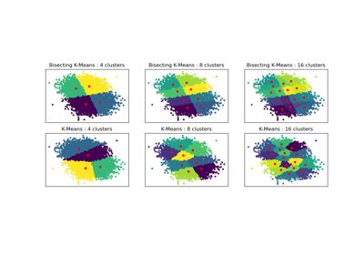
Bisecting K-Means and Regular K-Means Performance Comparison

Color Quantization using K-Means

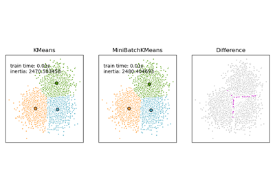
Comparison of the K-Means and MiniBatchKMeans clustering algorithms

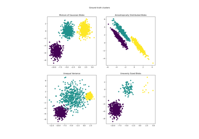
Demonstration of k-means assumptions

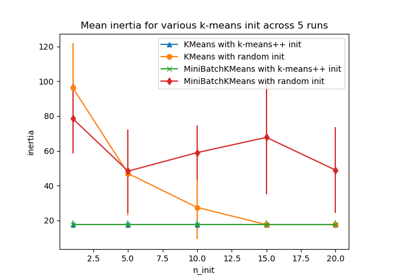
Empirical evaluation of the impact of k-means initialization

K-means Clustering

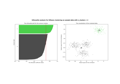
Selecting the number of clusters with silhouette analysis on KMeans clustering

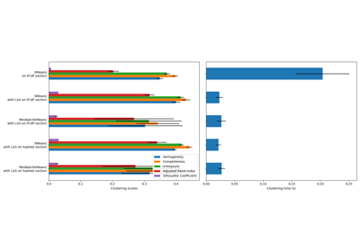
Clustering text documents using k-means

Comprehensive Learning Paths
150+ Hours of Videos
Complete Access to Jupyter notebooks, Datasets, References.

Machine Learning

K-means clustering algorithm from scratch.

April 26, 2020
Venmani A D

K-Means Clustering is an unsupervised learning algorithm that aims to group the observations in a given dataset into clusters. The number of clusters is provided as an input. It forms the clusters by minimizing the sum of the distance of points from their respective cluster centroids.

Basic Overview

Introduction to K-Means Clustering

Steps involved.

Maths Behind K-Means Clustering

Implementing K-Means from scratch

Elbow Method to find the optimal number of clusters

Grouping mall customers using K-Means

Basic overview of clustering.

Clustering is a type of unsupervised learning which is used to split unlabeled data into different groups.

Now, what does unlabeled data mean?

Unlabeled data means we don’t have a dependent variable (response variable) for the algorithm to compare as the ground truth. Clustering is generally used in Data Analysis to get to know about the different groups that may exist in our dataset.

We try to split the dataset into different groups, such that the data points in the same group have similar characteristics than the data points in different groups.

Now how to find whether the points are similar?

Use a good distance metric to compute the distance between a point and every other point. The points that have less distance are more similar. Euclidean distance is the most common metric.

Clustering algorithms are generally used in network traffic classification, customer, and market segmentation. It can be used on any tabular dataset, where you want to know which rows are similar to each other and form meaningful groups out of the dataset. First I am going to install the libraries that I will be using.

Let’s look into one of the most common clustering algorithms: K-Means in detail. Hands-on implementation on real project: Learn how to implement classification algorithms using multiple techniques in my Microsoft Malware Detection Project Course.

K-Means follows an iterative process in which it tries to minimize the distance of the data points from the centroid points. It’s used to group the data points into k number of clusters based on their similarity.

Euclidean distance is used to calculate the similarity.

Let’s see a simple example of how K-Means clustering can be used to segregate the dataset. In this example, I am going to use the make_blobs the command to generate isotropic gaussian blobs which can be used for clustering.

I passed in the number of samples to be generated to be 100 and the number of centers to be 5.

If you look at the value of y, you can see that the points are classified based on their clusters, but I won’t be using this compute the clusters, I will be using this only for evaluating purpose. For using K-Means you need to import KMeans from sklearn.cluster library.

For using KMeans, you need to specify the no of clusters as arguments. In this case, as we can look from the graph that there are 5 clusters, I will be passing 5 as arguments. But in general cases, you should use the Elbow Method to find the optimal number of clusters. I will be discussing this method in detail in the upcoming sections.

After passing the arguments, I have fitted the model and predicted the results. Now let’s visualize our predictions in a scatter plot.

There are 3 important steps in K-Means Clustering.

1. Initialize centroids – This is done by randomly choosing K no of points, the points can be present in the dataset or also random points.
2. Assign Clusters – The clusters are assigned to each point in the dataset by calculating their distance from the centroid and assigning it to the centroid with minimum distance.
3. Re-calculate the centroids – Updating the centroid by calculating the centroid of each cluster we have created.

Maths Behind K-Means Working

One of the few things that you need to keep in mind is that as we are using euclidean distance as the main parameter, it will be better to standardize your dataset if the x and y vary way too much like 10 and 100.

Also, it’s recommended to choose a wide range of points as initial clusters to check whether we are getting the same output, there is a possibility that you may get stuck at the local minimum rather than the global minimum.

Let’s use the same make_blobs example we used at the beginning. We will try to do the clustering without using the KMeans library.

I have set the K value to be 5 as before and also initialized the centroids randomly at first using the random.randint() function.

Then I am going to find the distance between the points. Euclidean distance is most commonly used for finding the similarity.

I have also stored all the minimum values in a variable minimum . Then I regrouped the dataset based on the minimum values we got and calculated the centroid value.

Then we need to repeat the above 2 steps over and over again until we reach the convergence.

Let’s plot it.

Elbow method to find the optimal number of clusters

One of the important steps in K-Means Clustering is to determine the optimal no. of clusters we need to give as an input. This can be done by iterating it through a number of n values and then finding the optimal n value.

For finding this optimal n, the Elbow Method is used.

You have to plot the loss values vs the n value and find the point where the graph is flattening, this point is considered as the optimal n value.

Let’s look at the example we have seen at first, to see the working of the elbow method. I am going to iterate it through a series of n values ranging from 1-20 and then plot their loss values.

I am going to be using the Mall_Customers Dataset. You can download the dataset from the given link

Let’s try to find if there are certain clusters between the customers based on their Age and Spending Score.

Predictive Modeling

How Naive Bayes Algorithm Works? (with example and full code)

Similar articles, complete introduction to linear regression in r, how to implement common statistical significance tests and find the p value, logistic regression – a complete tutorial with examples in r.

Subscribe to Machine Learning Plus for high value data science content

Machine Learning A-Z™: Hands-On Python & R In Data Science

Free sample videos:.

Office Hours
Python Tutorial
Markov Decisions
Practice Midterms
Midterm Solutions
Big Picture
Programming:
Driverless Car
Visual Cortex
Problem Sets:
Search Pset
Variable Pset
Learning Pset
Variable Models Pset
Machine Learning Pset
Final Project
Self Driving Car Machine Translation Deep Blue Watson

Written by Chris Piech. Based on a handout by Andrew Ng.

The Basic Idea

Say you are given a data set where each observed example has a set of features, but has no labels. Labels are an essential ingredient to a supervised algorithm like Support Vector Machines, which learns a hypothesis function to predict labels given features. So we can't run supervised learning. What can we do?

One of the most straightforward tasks we can perform on a data set without labels is to find groups of data in our dataset which are similar to one another -- what we call clusters.

K-Means is one of the most popular "clustering" algorithms. K-means stores $k$ centroids that it uses to define clusters. A point is considered to be in a particular cluster if it is closer to that cluster's centroid than any other centroid.

K-Means finds the best centroids by alternating between (1) assigning data points to clusters based on the current centroids (2) chosing centroids (points which are the center of a cluster) based on the current assignment of data points to clusters.

Figure 1: K-means algorithm. Training examples are shown as dots, and cluster centroids are shown as crosses. (a) Original dataset. (b) Random initial cluster centroids. (c-f) Illustration of running two iterations of k-means. In each iteration, we assign each training example to the closest cluster centroid (shown by "painting" the training examples the same color as the cluster centroid to which is assigned); then we move each cluster centroid to the mean of the points assigned to it. Images courtesy of Michael Jordan.

The Algorithm

In the clustering problem, we are given a training set ${x^{(1)}, ... , x^{(m)}}$, and want to group the data into a few cohesive "clusters." Here, we are given feature vectors for each data point $x^{(i)} \in \mathbb{R}^n$ as usual; but no labels $y^{(i)}$ (making this an unsupervised learning problem). Our goal is to predict $k$ centroids and a label $c^{(i)}$ for each datapoint. The k-means clustering algorithm is as follows:

Implementation

Here is pseudo-python code which runs k-means on a dataset. It is a short algorithm made longer by verbose commenting. # Function: K Means # ------------- # K-Means is an algorithm that takes in a dataset and a constant # k and returns k centroids (which define clusters of data in the # dataset which are similar to one another). def kmeans(dataSet, k): # Initialize centroids randomly numFeatures = dataSet.getNumFeatures() centroids = getRandomCentroids(numFeatures, k) # Initialize book keeping vars. iterations = 0 oldCentroids = None # Run the main k-means algorithm while not shouldStop(oldCentroids, centroids, iterations): # Save old centroids for convergence test. Book keeping. oldCentroids = centroids iterations += 1 # Assign labels to each datapoint based on centroids labels = getLabels(dataSet, centroids) # Assign centroids based on datapoint labels centroids = getCentroids(dataSet, labels, k) # We can get the labels too by calling getLabels(dataSet, centroids) return centroids # Function: Should Stop # ------------- # Returns True or False if k-means is done. K-means terminates either # because it has run a maximum number of iterations OR the centroids # stop changing. def shouldStop(oldCentroids, centroids, iterations): if iterations > MAX_ITERATIONS: return True return oldCentroids == centroids # Function: Get Random Centroids # ------------- # Returns k random centroids, each of dimension n. def getRandomCentroids(n, k): # return some reasonable randomization. --> # Function: Get Labels # ------------- # Returns a label for each piece of data in the dataset. def getLabels(dataSet, centroids): # For each element in the dataset, chose the closest centroid. # Make that centroid the element's label. # Function: Get Centroids # ------------- # Returns k random centroids, each of dimension n. def getCentroids(dataSet, labels, k): # Each centroid is the geometric mean of the points that # have that centroid's label. Important: If a centroid is empty (no points have # that centroid's label) you should randomly re-initialize it.

Important note: You might be tempted to calculate the distance between two points manually, by looping over values. This will work, but it will lead to a slow k-means! And a slow k-means will mean that you have to wait longer to test and debug your solution.

Let's define three vectors:

To calculate the distance between x and y we can use: np.sqrt(sum((x - y) ** 2))

To calculate the distance between all the length 5 vectors in z and x we can use: np.sqrt(((z-x)**2).sum(axis=0))

Expectation Maximization

K-Means is really just the EM (Expectation Maximization) algorithm applied to a particular naive bayes model.

To demonstrate this remarkable claim, consider the classic naive bayes model with a class variable which can take on discrete values (with domain size $k$) and a set of feature variables, each of which can take on a continuous value (see figure 2). The conditional probability distributions for $P(f_i = x | C= c)$ is going to be slightly different than usual. Instead of storing this conditional probability as a table, we are going to store it as a single normal (gaussian) distribution, with it's own mean and a standard deviation of 1. Specifically, this means that: $P(f_i = x | C= c) \sim \mathcal{N}(\mu_{c,i}, 1)$

Learning the values of $\mu_{c, i}$ given a dataset with assigned values to the features but not the class variables is the provably identical to running k-means on that dataset.

Figure 2: The K-Means algorithm is the EM algorithm applied to this Bayes Net.

If we know that this is the strcuture of our bayes net, but we don't know any of the conditional probability distributions then we have to run Parameter Learning before we can run Inference.

In the dataset we are given, all the feature variables are observed (for each data point) but the class variable is hidden. Since we are running Parameter Learning on a bayes net where some variables are unobserved, we should use EM.

Lets review EM. In EM, you randomly initialize your model parameters, then you alternate between (E) assigning values to hidden variables, based on parameters and (M) computing parameters based on fully observed data.

E-Step : Coming up with values to hidden variables, based on parameters. If you work out the math of chosing the best values for the class variable based on the features of a given piece of data in your data set, it comes out to "for each data-point, chose the centroid that it is closest to, by euclidean distance, and assign that centroid's label." The proof of this is within your grasp! See lecture.

M-Step : Coming up with parameters, based on full assignments. If you work out the math of chosing the best parameter values based on the features of a given piece of data in your data set, it comes out to "take the mean of all the data-points that were labeled as c."

So what? Well this gives you an idea of the qualities of k-means. Like EM, it is provably going to find a local optimum. Like EM, it is not necessarily going to find a global optimum. It turns out those random initial values do matter.

Figure 1 shows k-means with a 2-dimensional feature vector (each point has two dimensions, an x and a y). In your applications, will probably be working with data that has a lot of features. In fact each data-point may be hundreds of dimensions. We can visualize clusters in up to 3 dimensions (see figure 3) but beyond that you have to rely on a more mathematical understanding.

Figure 3: KMeans in other dimensions. (left) K-means in 2d. (right) K-means in 3d. You have to imagine k-means in 4d.

Statistics Made Easy

K-Means Clustering in R: Step-by-Step Example

Clustering is a technique in machine learning that attempts to find clusters of observations within a dataset.

The goal is to find clusters such that the observations within each cluster are quite similar to each other, while observations in different clusters are quite different from each other.

Clustering is a form of unsupervised learning because we’re simply attempting to find structure within a dataset rather than predicting the value of some response variable .

Clustering is often used in marketing when companies have access to information like:

Household income
Household size
Head of household Occupation
Distance from nearest urban area

When this information is available, clustering can be used to identify households that are similar and may be more likely to purchase certain products or respond better to a certain type of advertising.

One of the most common forms of clustering is known as k-means clustering .

What is K-Means Clustering?

K-means clustering is a technique in which we place each observation in a dataset into one of K clusters.

The end goal is to have K clusters in which the observations within each cluster are quite similar to each other while the observations in different clusters are quite different from each other.

In practice, we use the following steps to perform K-means clustering:

1. Choose a value for K .

First, we must decide how many clusters we’d like to identify in the data. Often we have to simply test several different values for K and analyze the results to see which number of clusters seems to make the most sense for a given problem.

2. Randomly assign each observation to an initial cluster, from 1 to K.

3. Perform the following procedure until the cluster assignments stop changing.

For each of the K clusters, compute the cluster centroid. This is simply the vector of the p feature means for the observations in the k th cluster.
Assign each observation to the cluster whose centroid is closest. Here, closest is defined using Euclidean distance .

K-Means Clustering in R

The following tutorial provides a step-by-step example of how to perform k-means clustering in R.

Step 1: Load the Necessary Packages

First, we’ll load two packages that contain several useful functions for k-means clustering in R.

Step 2: Load and Prep the Data

For this example we’ll use the USArrests dataset built into R, which contains the number of arrests per 100,000 residents in each U.S. state in 1973 for Murder , Assault , and Rape along with the percentage of the population in each state living in urban areas, UrbanPop .

The following code shows how to do the following:

Load the USArrests dataset
Remove any rows with missing values
Scale each variable in the dataset to have a mean of 0 and a standard deviation of 1

Step 3: Find the Optimal Number of Clusters

To perform k-means clustering in R we can use the built-in kmeans() function, which uses the following syntax:

kmeans(data, centers, nstart)

data: Name of the dataset.
centers: The number of clusters, denoted k .
nstart: The number of initial configurations. Because it’s possible that different initial starting clusters can lead to different results, it’s recommended to use several different initial configurations. The k-means algorithm will find the initial configurations that lead to the smallest within-cluster variation.

Since we don’t know beforehand how many clusters is optimal, we’ll create two different plots that can help us decide:

1. Number of Clusters vs. the Total Within Sum of Squares

First, we’ll use the fviz_nbclust() function to create a plot of the number of clusters vs. the total within sum of squares:

Optimal number of clusters in k-means clustering

Typically when we create this type of plot we look for an “elbow” where the sum of squares begins to “bend” or level off. This is typically the optimal number of clusters.

For this plot it appears that there is a bit of an elbow or “bend” at k = 4 clusters.

2. Number of Clusters vs. Gap Statistic

Another way to determine the optimal number of clusters is to use a metric known as the gap statistic , which compares the total intra-cluster variation for different values of k with their expected values for a distribution with no clustering.

We can calculate the gap statistic for each number of clusters using the clusGap() function from the cluster package along with a plot of clusters vs. gap statistic using the fviz_gap_stat() function:

Gap statistic for optimal number of clusters

From the plot we can see that gap statistic is highest at k = 4 clusters, which matches the elbow method we used earlier.

Step 4: Perform K-Means Clustering with Optimal K

Lastly, we can perform k-means clustering on the dataset using the optimal value for k of 4:

From the results we can see that:

16 states were assigned to the first cluster
13 states were assigned to the second cluster
13 states were assigned to the third cluster
8 states were assigned to the fourth cluster

We can visualize the clusters on a scatterplot that displays the first two principal components on the axes using the fivz_cluster() function:

We can also use the aggregate() function to find the mean of the variables in each cluster:

We interpret this output is as follows:

The mean number of murders per 100,000 citizens among the states in cluster 1 is 3.6 .
The mean number of assaults per 100,000 citizens among the states in cluster 1 is 78.5 .
The mean percentage of residents living in an urban area among the states in cluster 1 is 52.1% .
The mean number of rapes per 100,000 citizens among the states in cluster 1 is 12.2 .

We can also append the cluster assignments of each state back to the original dataset:

Pros & Cons of K-Means Clustering

K-means clustering offers the following benefits:

It is a fast algorithm.
It can handle large datasets well.

However, it comes with the following potential drawbacks:

It requires us to specify the number of clusters before performing the algorithm.
It’s sensitive to outliers.

Two alternatives to k-means clustering are k-medoids clustering and hierarchical clustering .

You can find the complete R code used in this example here .

Featured Posts

5 Regularization Techniques You Should Know

Hey there. My name is Zach Bobbitt. I have a Masters of Science degree in Applied Statistics and I’ve worked on machine learning algorithms for professional businesses in both healthcare and retail. I’m passionate about statistics, machine learning, and data visualization and I created Statology to be a resource for both students and teachers alike. My goal with this site is to help you learn statistics through using simple terms, plenty of real-world examples, and helpful illustrations.

8 Replies to “K-Means Clustering in R: Step-by-Step Example”

Excellent, thank you!

Could you please clarify that how nstart is selected as 25 here?

Hi, could you tell me please, how can I have the data set of the cretaed clusters, so I can know which values are in each cluster?

Thank you very much. Statology is a very valuable resource. Sincerely,

Hi ! Thank a lot this work.

so, I just want to know how did you do for conversing the character column to column numeric ( the atribut of city)

How does one interpret Dim1 and Dim2 in the cluster plot?

I tried to run many of the models in R coded under machine learning and almost all of them failed. I am using the current version of R.

Thanks for your sharing

Join the Statology Community

I have read and agree to the terms & conditions

Homework 4: K-Means Clustering

Part I Due : at 11:59pm on Tuesday, February 8, 2022. Submit via Gradescope. (REQUIRED Feedback Survey ) Part II Due : at 11:59pm on Monday, February 14, 2022. Submit via Gradescope. (REQUIRED Feedback Survey )

For Part I you will submit kmeans.py with at least Part 1 completed. You will not necessarily get any feedback on Part I before Part II is due, so do not wait to get started on Part II. What you submit for the Part I deadline will not be graded for style at that time - but of course we recommend that you go ahead and use good style!
For Part II you will re-submit kmeans.py and submit analysis.py with everything (Parts 1 and 2) completed and with good style. At that time we will grade the entire homework for correctness and style. If you made a mistake in Part I, please fix those mistakes before submitting Part II so you do not lose points on them twice.
Your overall grade for this homework will come approximately 25% from Part I and 75% from Part II. Overall HW4 will count as approximately 1.5 homeworks.
For all of our assignments you should NOT use parts of Python not yet discussed in class or the course readings. In addition, do not use the functions: min , max , or sum .

Learning Objectives:

Implement a popular clustering algorithm for data analysis
Practice using lists and dictionaries for computational problem solving

This time we have a couple videos available to help clarify the assignment. We highly recommend watching these videos before starting, or if you are confused about the content.

The videos will also be embedded here:

The Algorithm

Part 0: getting started, part 1: implementing the algorithm, step 1: calculating euclidean distances, step 2: assigning data points to closest centroids, step 3: update assignment of points to centroids, step 4: update centroids, step 5: clustering 2d points, step 6: submit, step 1: load the final centroids: what happened, step 2: rewrite update_assignment, step 3: calculate the count of the majority label, step 4: calculate the accuracy of the algorithm, step 5: run analysis and think about the results, step 6: final submit, introduction.

In Homework 4, we will implement a commonly-used algorithm: K-means clustering. (Read more about K-means on the K-means Wikipedia page if you're interested). K-means is a popular machine learning and data mining algorithm that discovers potential clusters within a dataset. Finding these clusters in a dataset can often reveal interesting and meaningful structures underlying the distribution of data. K-means clustering has been applied to many problems in science and still remains popular today for its simplicity and effectiveness. Here are a few examples of recently published papers using K-means:

(Computer Science) Hand-written digit recognition (We will do this in Part 2!)
(Natural Language Processing) Categorizing text based on clusters
(Biology) Discovering gene expression networks

Hopefully, these examples motivate you to try this homework out! You will very likely be able to apply this computational tool to some problems relevant to you! We will break down the name and explain the algorithm now.

Background: Data, Distances, Clusters and Centroids

We will assume we have a dataset of m data points where each data point is n -dimensional. For example, we could have 100 points on a two dimensional plane, then m = 100 and n = 2.

Euclidean Distance

$assignments k means$

This is commonly known as the Euclidean distance . For example, if we had the three-dimensional points x1 and x2 defined as Python lists:

x1 = [-2, -1, -4] x2 = [10, -5, 5]

$assignments k means$

Here is another example with two four-dimensional points:

$assignments k means$

A cluster is a collection of points that are part of the same group. For k-means, every point has a cluster that it is part of. As the algorithm progresses, points may change what cluster they are currently in, even though the point itself does not move.

For instance, all blue points are part of cluster1 , all red points are part of cluster2 , all green points are part of cluster3

$assignments k means$

For example, if a cluster contains three 2D points (displayed as Python lists) as below: x1 = [1, 1] x2 = [2, 3] x3 = [3, 2] The centroid for this cluster is defined as: c = [(1 + 2 + 3)/3, (1 + 3 + 2)/3] # evaluates to [2, 2]

Our ultimate goal is to partition the data points into K clusters. How do we know which data point belongs to which cluster? In K-means, we assign each data point to the cluster whose centroid is closest to that data point.

First, we assign all data points to their corresponding centroids by finding the centroid that is closest.
Then, we adjust the centroid location to be the average of all points in that cluster.

We iteratively repeat these two steps to achieve better and better cluster centroids and meaningful assignments of data points.

Note that the data points do not change! Only the location of the centroids change with each iteration (and thus the points that are closest to each centroid changes).

K-means Convergence

One last question you may have is, when do we stop repeating these two steps? I.e., what does it mean for the algorithm to have converged? We say the algorithm has converged if the locations of all centroids did not change much between two iterations. (ex. Within 1 * 10 -5 or 0.00001)

Take this example of two centroids of 2-dimensional points. If at the previous iteration, we have the two centroid locations as: c1 = [0.45132, -0.99134] c2 = [-0.34135, -2.3525] And at the next iteration the centroids are updated to: c1 = [1.43332, -1.9334] c2 = [-1.78782, -2.3523] Then we say the algorithm has NOT converged, since the location of the two centroids are very different between iterations. However, if the new locations of the centroids are instead: c1 = [0.45132, -0.99134] c2 = [-0.34135, -2.3524] Then we say the algorithm HAS converged, since the locations of the two centroids are very similar between iterations (Typically, "very similar" means for every dimension of two points a and b, their difference (|a - b|) is smaller than some constant (1 * 10 -5 or 0.00001 is a common choice)).

In summary, the K-means algorithm (in pseudo code) is described as follows:

First, data points are assigned to whichever centroid is closest (and colored accordingly),
Then centroid locations are adjusted based on the mean of all red/blue points.

In the following parts of this homework, you will implement this algorithm and apply it to (1) 2D points shown in the gif above; (2) a small subset of the MNIST hand-written digit dataset.

Download homework4.zip and unzip the file to get started. You should see the following file structure in the homework4 folder:

The red highlighted parts are where you will work on your code. We have provided utils.py which contains helper code to help you complete the assignment. Do not change anything in utils.py !

data : A list of data points, where each data point is a list of floats. Example: data = [[0.34, -0.2, 1.13, 4.3], [5.1, -12.6, -7.0, 1.9], [-15.7, 0.06, -7.1, 11.2]] Here, data contains three data points, where each data point is four-dimensional. (In this example point 1 is [0.34, -0.2, 1.13, 4.3], point 2 is [5.1, -12.6, -7.0, 1.9] and point 3 is [-15.7, 0.06, -7.1, 11.2])
centroids : A dictionary of centroids, where the keys are strings (centroid names) and the values are lists (centroid locations) Example: centroids = {"centroid1": [1.1, 0.2, -3.1, -0.4], "centroid2": [9.3, 6.1, -4.7, 0.18]} Here, centroids contains two key-value pairs, where key is the centroid name, and value is the location of the centroid. You should NOT change the names of the centroids when you later update their locations.

Implement the following function in kmeans.py :

If you want more information on what Euclidean distance is, re-read the Euclidean distance background section in the spec and/or the Euclidean distance Wikipedia page . In the code we have provided you for this (and all functions you need to implement), the body of the function is empty. We have provided testing code for you to verify your implementation. Run python kmeans.py in a terminal window to verify your implementation of euclidean_distance . If you passed our tests, you should see: test_euclidean_distance passed. Note that you may find several assertions further down in the program failing at this point. This is to be expected since you have not implemented those parts of the program yet! In fact this will continue to happen as you progress through the problems. Success usually means you are no longer failing the same assertion, but that instead a different assertion is failing further down in the program.

If you want more information on centroids, check out the Centroids section in the spec. We have provided testing code for you to verify your implementation. test_closest_centroid() is already set up to run when python kmeans.py is typed in a terminal window. Check the output of this test to verify your implementation.

Notice that your algorithm should run regardless of if any centroid becomes empty, i.e. there are no points that are the closest to a centroid. In that case you should not include that centroid in the dictionary you return. We have provided testing code for you to verify your implementation. test_update_assignment() is already set up to run when python kmeans.py is typed in a terminal window. Check the output of this test to verify your implementation.

Notice that you should not hard-code the dimensionality of data - your code needs to run regardless of the dimension of data!

We have provided testing code for you to verify your implementation. test_mean_of_points() is already set up to run when python kmeans.py is typed in a terminal window. Check the output of this test to verify your implementation. A common error students make when implementing this function is to modify the provided list of points. Be sure your implementation does not modify the provided list of points. Now implement the following function in kmeans.py :

Notice that you should not hard-code the dimensionality of data - your code needs to run regardless of the dimension of data! We have provided testing code for you to verify your implementation. test_update_centroids() is already set up to run when python kmeans.py is typed in a terminal window. Check the output of this test to verify your implementation. You have now completed all parts needed to run your k-means algorithm! As a sanity check, try running everything together one more time by typing: python kmeans.py in the terminal window. You should see: All tests passed.

You have now completed all parts needed to run your k-means algorithm! Now, let's verify your implementation by running the algorithm on 2D points. At the bottom of kmeans.py you should see code like this:

This is the code that actually runs when you run this file. Right now your code is only calling the main_test() function. De-comment the last four lines and turn the call to main_test() into a comment . These new commands will load the 2D data points and the initial centroids we provided in from .csv files. After that, main_2d will execute the k-means algorithm and write_centroids_tofile will save the final centroids to a file to save them permanently. Your code should now look like this:

Now run your program again by typing python kmeans.py in the terminal window. If you are successful, you should see: K-means converged after 7 steps. as the output of the program. In addition, there should be 7 plots generated, in the results/2D/ folder. If you examine these 7 plots, they should be identical to the steps shown in the the gif shown in the algorithm section of this spec .

You've completed part 1! Before you take a break, be sure to submit kmeans.py via Gradescope . To ensure your program produces the correct output, you should make the code at the bottom of your kmeans.py look identical to what we described in Step 5.

Answer a REQUIRED survey asking how much time you spent and other reflections on this part of the assignment.

Part 2: Another dataset & Analyzing the Performance

Trying the algorithm on mnist.

Now that you have successfully run K-means clustering on 2-dimensional data points with 2 centroids, we will use your code to do clustering of 784-dimensional data points with 10 centroids. Don't worry, you won't need to change any of the code that you wrote!

Each of these images is 28 pixels by 28 pixels, for a total of 784 pixels. (As in HW3, pixels have values between 0 and 255 (0=black, 255=white), although we don't need to know this for K-means.) Each image can be thought of as a 784-dimensional data point, represented as a list containing 784 numbers. For the images shown above, many of the numbers would be zero since the image is mostly black. So the nine sample images above are actually nine sample data points!

We will see how applying K-means to these digit images helps us discover clusters of images which contain mostly one kind of digit!

To load the MNIST dataset instead of the 2D points, change the code at the bottom of the file to the following (the red text shows the changes that should be made):

You should leave the rest of your code intact, and it should run with the new data without errors! Run this command again (it may take a minute to run on this data set!):

Analyzing the Performance

How do we evaluate the performance of our algorithm? The images in the MNIST data set have been labelled with the digit they actually represent. (You can see this label as the digit in the first column on each row in the file mnist.csv . Each row of that file represents one data point (image).) So, one way to evaluate our algorithm would be to examine the accuracy of the classification of the images from MNIST. For example, how many of the images known to be (labelled as) the digit 4 ended up in the centroid we think of as representing the digit 4? First, let's define the "classifications" of our data points provided by K-means. We take a majority-takes-all approach: we assign each cluster a label as the majority labels of all data points in this cluster. For example, say we have data points with these labels assigned to cluster1: 2, 2, 2, 2, 2, 2, 8, 6, 2, 2, 6, 8, 8, 2, 2 Since there are 10 2's, 3 8's, and 2 6's, we say the label of cluster 1 is 2 since it's the majority label. (i.e The first six images have a label of 2, the seventh image has a label of 8, the eighth image has a label of 6)

$assignments k means$

Now we can start the analysis. We have provided the code for you near the bottom of analysis.py :

First, please take a closer look at this centroids dictionary and/or the images that were generated. Feel free to write some print statements to explore the content (you don't need to show this code when you submit your homework) - how many centroids are there in the dictionary now? In Part A, we initialized the algorithm with 10 randomly chosen positions as the initial centroids. Why are there fewer centroids than 10 now? What do you suspect happened? >This question is just for fun (un-graded), but we want you to at least think about what is happening and give an answer. Leave your answers as comments at the bottom of the file ( analysis.py ) . Please do not stress about these questions! There is no need to do anything for this question other than think about it.

When we implemented the update_assignment function, it assigned each data point to the centroid it is closest to. This works great for our algorithm, but now we are not only interested in which centroid the data point is assigned to, but also the true label of that data point in order to perform the accuracy analysis. Therefore, we need to update the function to incorporate more parameters and return different values. Implement the following function in analysis.py :

Notice the red parts as the difference between the previous version of the function you wrote and what you need to write now. Instead of nested lists of data points as the values of the dictionary returned, it should now be single lists that contain the labels of the data points, not the actual data points . Feel free to copy your previous implementation in kmeans.py over as a starting point. And just like your old implementation, you should use the get_closest_centroid function when implementing this one. We have provided testing code for you to verify your implementation. De-comment the call to main_test() near the bottom of analysis.py and then run python analysis.py , which will call that same main_test(). Similar to part 1, you should see test_update_assignment passed if your update_assignment is working. You will see a test fail after that, since your other functions are not ready yet.

In the next function, you should take in a single list of labels, and return the count of the majority label defined as above. Implement the following function in analysis.py :

We have provided testing code for you to verify your implementation. Run python analysis.py again. This time you should see test_majority_count passed if your majority_count is working. You will see a test fail after that, since your last function is not ready yet.

Use the two functions you implemented in the previous parts of Part 2 to calculate the accuracy for every cluster and the whole algorithm, defined as above in the Analyzing the Performance section . Implement the following function in analysis.py :

We have provided testing code for you to verify your implementation. Run python analysis.py again. This time you should see test_accuracy passed if your accuracy function is working. Now you should also see all tests passed.

You have now completed all the parts required to run the analysis. Please de-comment the last few commented lines of code at the bottom of analysis.py and comment out the call to main_test() (and remove your exploration code from Step 1) so you have:

And run the program by typing: python analysis.py Note that the file name returned in the output does not necessarily correspond with the label assigned to the digit (ex. centroid0.png is not necessarily an image of '0'). Instead, decide on the label of the image by looking at the returned image itself. What is the output? Is this value surprising? It might be helpful to take another look at the final centroid images from MNIST in the results/MNIST/final folder -- In your opinion, based on these centroids, which digits are easier to be distinguished by the algorithm, and which are harder? If you can't tell from the centroid images, consider printing the accuracy for each label inside of your accuracy function. This question is graded, but don't stress too much about it . Reasonable answers will receive full credit. (ie 2-3 sentences). Leave your answer as comments at the bottom of the file analysis.py . There is no need to do anything for this question other than think about it.

Be sure to submit both analysis.py and kmeans.py via Gradescope under part 2.

Partitional Clustering in R: The Essentials

K-Means Clustering in R: Algorithm and Practical Examples

K-means clustering (MacQueen 1967) is one of the most commonly used unsupervised machine learning algorithm for partitioning a given data set into a set of k groups (i.e. k clusters ), where k represents the number of groups pre-specified by the analyst. It classifies objects in multiple groups (i.e., clusters), such that objects within the same cluster are as similar as possible (i.e., high intra-class similarity ), whereas objects from different clusters are as dissimilar as possible (i.e., low inter-class similarity ). In k-means clustering, each cluster is represented by its center (i.e, centroid ) which corresponds to the mean of points assigned to the cluster.

In this article, you will learn:

The basic steps of k-means algorithm
How to compute k-means in R software using practical examples
Advantages and disavantages of k-means clustering

K-means basic ideas

K-means algorithm, required r packages and functions, estimating the optimal number of clusters, computing k-means clustering, accessing to the results of kmeans() function, visualizing k-means clusters, k-means clustering advantages and disadvantages, alternative to k-means clustering, related book.

The basic idea behind k-means clustering consists of defining clusters so that the total intra-cluster variation (known as total within-cluster variation) is minimized.

There are several k-means algorithms available. The standard algorithm is the Hartigan-Wong algorithm (Hartigan and Wong 1979) , which defines the total within-cluster variation as the sum of squared distances Euclidean distances between items and the corresponding centroid:

\[ W(C_k) = \sum\limits_{x_i \in C_k} (x_i - \mu_k)^2 \]

$x_i$ design a data point belonging to the cluster $C_k$
$\mu_k$ is the mean value of the points assigned to the cluster $C_k$

Each observation ( $x_i$ ) is assigned to a given cluster such that the sum of squares (SS) distance of the observation to their assigned cluster centers $\mu_k$ is a minimum.

We define the total within-cluster variation as follow:

\[ tot.withinss = \sum\limits_{k=1}^k W(C_k) = \sum\limits_{k=1}^k \sum\limits_{x_i \in C_k} (x_i - \mu_k)^2 \]

The total within-cluster sum of square measures the compactness (i.e goodness ) of the clustering and we want it to be as small as possible.

The first step when using k-means clustering is to indicate the number of clusters (k) that will be generated in the final solution.

The algorithm starts by randomly selecting k objects from the data set to serve as the initial centers for the clusters. The selected objects are also known as cluster means or centroids.

Next, each of the remaining objects is assigned to it’s closest centroid, where closest is defined using the Euclidean distance between the object and the cluster mean. This step is called “cluster assignment step”. Note that, to use correlation distance, the data are input as z-scores.

After the assignment step, the algorithm computes the new mean value of each cluster. The term cluster “centroid update” is used to design this step. Now that the centers have been recalculated, every observation is checked again to see if it might be closer to a different cluster. All the objects are reassigned again using the updated cluster means.

The cluster assignment and centroid update steps are iteratively repeated until the cluster assignments stop changing (i.e until convergence is achieved). That is, the clusters formed in the current iteration are the same as those obtained in the previous iteration.

K-means algorithm can be summarized as follow:

Specify the number of clusters (K) to be created (by the analyst)
Select randomly k objects from the dataset as the initial cluster centers or means
Assigns each observation to their closest centroid, based on the Euclidean distance between the object and the centroid
For each of the k clusters update the cluster centroid by calculating the new mean values of all the data points in the cluster. The centoid of a K t h cluster is a vector of length p containing the means of all variables for the observations in the k t h cluster; p is the number of variables.
Iteratively minimize the total within sum of square. That is, iterate steps 3 and 4 until the cluster assignments stop changing or the maximum number of iterations is reached. By default, the R software uses 10 as the default value for the maximum number of iterations.

Computing k-means clustering in R

We’ll use the demo data sets “USArrests”. The data should be prepared as described in chapter @ref(data-preparation-and-r-packages). The data must contains only continuous variables, as the k-means algorithm uses variable means. As we don’t want the k-means algorithm to depend to an arbitrary variable unit, we start by scaling the data using the R function scale() as follow:

The standard R function for k-means clustering is kmeans () [ stats package], which simplified format is as follow:

x : numeric matrix, numeric data frame or a numeric vector
centers : Possible values are the number of clusters (k) or a set of initial (distinct) cluster centers. If a number, a random set of (distinct) rows in x is chosen as the initial centers.
iter.max : The maximum number of iterations allowed. Default value is 10.
nstart : The number of random starting partitions when centers is a number. Trying nstart > 1 is often recommended.

To create a beautiful graph of the clusters generated with the kmeans () function, will use the factoextra package.

Installing factoextra package as:
Loading factoextra :

The k-means clustering requires the users to specify the number of clusters to be generated.

One fundamental question is: How to choose the right number of expected clusters (k)?

Different methods will be presented in the chapter “cluster evaluation and validation statistics”.

Here, we provide a simple solution. The idea is to compute k-means clustering using different values of clusters k. Next, the wss (within sum of square) is drawn according to the number of clusters. The location of a bend (knee) in the plot is generally considered as an indicator of the appropriate number of clusters.

The R function fviz_nbclust () [in factoextra package] provides a convenient solution to estimate the optimal number of clusters.

The plot above represents the variance within the clusters. It decreases as k increases, but it can be seen a bend (or “elbow”) at k = 4. This bend indicates that additional clusters beyond the fourth have little value.. In the next section, we’ll classify the observations into 4 clusters.

As k-means clustering algorithm starts with k randomly selected centroids, it’s always recommended to use the set.seed() function in order to set a seed for R’s random number generator . The aim is to make reproducible the results, so that the reader of this article will obtain exactly the same results as those shown below.

The R code below performs k-means clustering with k = 4:

As the final result of k-means clustering result is sensitive to the random starting assignments, we specify nstart = 25 . This means that R will try 25 different random starting assignments and then select the best results corresponding to the one with the lowest within cluster variation. The default value of nstart in R is one. But, it’s strongly recommended to compute k-means clustering with a large value of nstart such as 25 or 50, in order to have a more stable result.

The printed output displays:

the cluster means or centers: a matrix, which rows are cluster number (1 to 4) and columns are variables
the clustering vector: A vector of integers (from 1:k) indicating the cluster to which each point is allocated

It’s possible to compute the mean of each variables by clusters using the original data:

If you want to add the point classifications to the original data, use this:

kmeans() function returns a list of components, including:

cluster : A vector of integers (from 1:k) indicating the cluster to which each point is allocated
centers : A matrix of cluster centers (cluster means)
totss : The total sum of squares (TSS), i.e $\sum{(x_i - \bar{x})^2}$ . TSS measures the total variance in the data.
withinss : Vector of within-cluster sum of squares, one component per cluster
tot.withinss : Total within-cluster sum of squares, i.e. $sum(withinss)$
betweenss : The between-cluster sum of squares, i.e. $totss - tot.withinss$
size : The number of observations in each cluster

These components can be accessed as follow:

It is a good idea to plot the cluster results. These can be used to assess the choice of the number of clusters as well as comparing two different cluster analyses.

Now, we want to visualize the data in a scatter plot with coloring each data point according to its cluster assignment.

The problem is that the data contains more than 2 variables and the question is what variables to choose for the xy scatter plot.

A solution is to reduce the number of dimensions by applying a dimensionality reduction algorithm, such as Principal Component Analysis (PCA) , that operates on the four variables and outputs two new variables (that represent the original variables) that you can use to do the plot.

In other words, if we have a multi-dimensional data set, a solution is to perform Principal Component Analysis (PCA) and to plot data points according to the first two principal components coordinates.

The function fviz_cluster () [ factoextra package] can be used to easily visualize k-means clusters. It takes k-means results and the original data as arguments. In the resulting plot, observations are represented by points, using principal components if the number of variables is greater than 2. It’s also possible to draw concentration ellipse around each cluster.

K-means clustering is very simple and fast algorithm. It can efficiently deal with very large data sets. However there are some weaknesses, including:

It assumes prior knowledge of the data and requires the analyst to choose the appropriate number of cluster (k) in advance
The final results obtained is sensitive to the initial random selection of cluster centers. Why is it a problem? Because, for every different run of the algorithm on the same dataset, you may choose different set of initial centers. This may lead to different clustering results on different runs of the algorithm.
It’s sensitive to outliers.
If you rearrange your data, it’s very possible that you’ll get a different solution every time you change the ordering of your data.

Possible solutions to these weaknesses, include:

Solution to issue 1: Compute k-means for a range of k values, for example by varying k between 2 and 10. Then, choose the best k by comparing the clustering results obtained for the different k values.
Solution to issue 2: Compute K-means algorithm several times with different initial cluster centers. The run with the lowest total within-cluster sum of square is selected as the final clustering solution.
To avoid distortions caused by excessive outliers, it’s possible to use PAM algorithm, which is less sensitive to outliers.

A robust alternative to k-means is PAM, which is based on medoids. As discussed in the next chapter, the PAM clustering can be computed using the function pam () [ cluster package]. The function pamk ( ) [fpc package] is a wrapper for PAM that also prints the suggested number of clusters based on optimum average silhouette width.

K-means clustering can be used to classify observations into k groups, based on their similarity. Each group is represented by the mean value of points in the group, known as the cluster centroid.

K-means algorithm requires users to specify the number of cluster to generate. The R function kmeans () [ stats package] can be used to compute k-means algorithm. The simplified format is kmeans(x, centers), where “x” is the data and centers is the number of clusters to be produced.

After, computing k-means clustering, the R function fviz_cluster () [ factoextra package] can be used to visualize the results. The format is fviz_cluster(km.res, data), where km.res is k-means results and data corresponds to the original data sets.

Hartigan, JA, and MA Wong. 1979. “Algorithm AS 136: A K-means clustering algorithm.” Applied Statistics . Royal Statistical Society, 100–108.

MacQueen, J. 1967. “Some Methods for Classification and Analysis of Multivariate Observations.” In Proceedings of the Fifth Berkeley Symposium on Mathematical Statistics and Probability, Volume 1: Statistics , 281–97. Berkeley, Calif.: University of California Press. http://projecteuclid.org:443/euclid.bsmsp/1200512992 .

Recommended for you

This section contains best data science and self-development resources to help you on your path.

Coursera - Online Courses and Specialization

Data science.

Course: Machine Learning: Master the Fundamentals by Stanford
Specialization: Data Science by Johns Hopkins University
Specialization: Python for Everybody by University of Michigan
Courses: Build Skills for a Top Job in any Industry by Coursera
Specialization: Master Machine Learning Fundamentals by University of Washington
Specialization: Statistics with R by Duke University
Specialization: Software Development in R by Johns Hopkins University
Specialization: Genomic Data Science by Johns Hopkins University

Popular Courses Launched in 2020

Google IT Automation with Python by Google
AI for Medicine by deeplearning.ai
Epidemiology in Public Health Practice by Johns Hopkins University
AWS Fundamentals by Amazon Web Services

Trending Courses

The Science of Well-Being by Yale University
Google IT Support Professional by Google
Python for Everybody by University of Michigan
IBM Data Science Professional Certificate by IBM
Business Foundations by University of Pennsylvania
Introduction to Psychology by Yale University
Excel Skills for Business by Macquarie University
Psychological First Aid by Johns Hopkins University
Graphic Design by Cal Arts

Amazing Selling Machine

Free Training - How to Build a 7-Figure Amazon FBA Business You Can Run 100% From Home and Build Your Dream Life! by ASM

Books - Data Science

Practical Guide to Cluster Analysis in R by A. Kassambara (Datanovia)
Practical Guide To Principal Component Methods in R by A. Kassambara (Datanovia)
Machine Learning Essentials: Practical Guide in R by A. Kassambara (Datanovia)
R Graphics Essentials for Great Data Visualization by A. Kassambara (Datanovia)
GGPlot2 Essentials for Great Data Visualization in R by A. Kassambara (Datanovia)
Network Analysis and Visualization in R by A. Kassambara (Datanovia)
Practical Statistics in R for Comparing Groups: Numerical Variables by A. Kassambara (Datanovia)
Inter-Rater Reliability Essentials: Practical Guide in R by A. Kassambara (Datanovia)
R for Data Science: Import, Tidy, Transform, Visualize, and Model Data by Hadley Wickham & Garrett Grolemund
Hands-On Machine Learning with Scikit-Learn, Keras, and TensorFlow: Concepts, Tools, and Techniques to Build Intelligent Systems by Aurelien Géron
Practical Statistics for Data Scientists: 50 Essential Concepts by Peter Bruce & Andrew Bruce
Hands-On Programming with R: Write Your Own Functions And Simulations by Garrett Grolemund & Hadley Wickham
An Introduction to Statistical Learning: with Applications in R by Gareth James et al.
Deep Learning with R by François Chollet & J.J. Allaire
Deep Learning with Python by François Chollet

Comments ( 2 )

how we can get data

The demo data used in this tutorial is available in the default installation of R. Juste type data(“USArrests”)

Give a comment Cancel reply

Course curriculum.

K-Means Clustering in R: Algorithm and Practical Examples 50 mins
K-Medoids in R: Algorithm and Practical Examples 35 mins
CLARA in R : Clustering Large Applications 35 mins

Alboukadel Kassambara

Role : founder of datanovia.

Website : https://www.datanovia.com/en
Experience : >10 years
Specialist in : Bioinformatics and Cancer Biology

Pair programming. On this assignment, you are encouraged (not required) to work with a partner provided you practice pair programming. Pair programming "is a practice in which two programmers work side-by-side at one computer, continuously collaborating on the same design, algorithm, code, or test." One partner is driving (designing and typing the code) while the other is navigating (reviewing the work, identifying bugs, and asking questions). The two partners switch roles every 30-40 minutes, and on demand, brainstorm.

Before pair programming, you must read the article All I really need to know about pair programming I learned in kindergarten . You should choose a partner of similar ability.

Only one partner submits the code and readme.txt ; the other partner submits only an abbrievated readme.txt that contains both partners' names, logins and information about extra credit. The names and logins of both partners MUST appear at the top of every submitted file. Both partners receive the same grade.

Writing code with a partner without following the pair programming instructions listed above is a serious violation of the course collaboration policy.

Initialize K centroids (See "Progress steps and testing" below). In our case, a centroid is just the average of all genes in a cluster, and it can be represented just like a normal gene.
Assign each gene to the cluster that has the closest centroid.
After all genes have been assigned to clusters, recalculate the centroids for each cluster (as averages of all genes in the cluster).
Repeat the gene assignments and centroid calculations until no change in gene assignment occurs between iterations .

Distance Measures. You will use two distance measures for clustering: Euclidean distance and Spearman rank correlation. Euclidean distance measures differences in the absolute levels of gene expression, whereas correlation compares the shapes of expression patterns. Furthermore, Spearman rank correlation uses ranks in place of absolute values, which makes it less sensitive to outliers (extremely high or low values) in the data.

For example, suppose we have two vectors x = [4.6, 1.9, 2.4] and y = [2.2, 6.6, 5.5]. Then the rank transforms of these two vectors would be r = [3, 1, 2] and s = [1, 3, 2], making d = [3-1, 1-3, 2-2] = [2, -2, 0].

Note that these functions should return distance measures; that is, the returned value should be high if the two vectors are dissimilar, low if they are similar, and zero if they are completely identical. This requirement is already met for Euclidean distance, but Spearman rank correlation varies between -1 and 1, and high values indicate similarity. Therefore, you must transform the Spearman rank correlation so that the returned value is always greater than or equal to zero, with high values indicating dissimilarity.

Overview of the code. The code is divided into several classes to represent our real-world data. These classes are Gene.java , Cluster.java , and KMeans.java . We have provided you with a start on each of these classes. As you read the following descriptions, refer to the relevant code files to get a sense of the structure of the program and to figure out the code we provided.

The Gene object will contain a gene name and an array of microarray expression levels. Gene objects will also have the ability to calculate the distance to another Gene . Gene also contains two member functions hashCode() and equals(Object o) for defining how to compare two objects of type Gene .
The Cluster object will contain a HashSet (more on this later) of Gene objects. Cluster objects will have the ability to print out the names of all the genes in the cluster, to calculate the centroid of the cluster, and to create an image that represents the cluster (this code is provided for you).
The KMeans class will contain an array of all the Gene objects to be clustered and an array of the Cluster objects created; it will also locally create arrays containing the centroids of the clusters. KMeans will also hold the main() function and all of the code to perform the clustering.

We're keeping the Gene objects in each Cluster in a HashSet<Gene> . The size of our clusters will change as we add genes to the cluster with nearest centroid. The generic class HashSet is part of the Java language specification (i.e. the standard libraries). A HashSet is an unordered set storing only unique elements, which means no duplicate elements can be present in the hash set. To enforce this uniqueness property, HashSet requires the containing member type to define hashCode() and equals(Object o) for checking equivalence of elements in the set. Once these are defined, inserting an element that is already present in the HashSet should have no effect.

All standard Java data types (such as Integer , String ) already have equals() and hashCode() defined, but not for user-defined classes such as Gene . For this assignment, you will need to define hashCode() and equals(Object o) for type Gene . Two Gene objects are considered equal if their gene names are equal. hashCode() returns an int that is the index of the "bin" a Gene object should be hashed to. You can assume hashCode() for Gene works in the same way as how hashCode() for gene name (of type String ) works.

Another method of HashSet that you want to be familiar with is add(Gene o) . The add(Gene o) method will take a Gene as an argument and add it to the hash set.

for (Gene gene : geneSet) { System.out.println(gene.getName()); }

We use the HashSet data structure to represent genes in a cluster, rather than array, for the reason of efficient equality checking between clusters, because the equality can be checked by finding the intersections of two HashSet s. If the size of intersection is equal to the size of cluster, then the two clusters are equal. At each iteration, you need to check for equality between the cluster before iteration and the cluster after iteration, for every cluster in the list, and terminate the iterative algorithm only if all clusters do not change. You can check for equality of two sets by: s1.containsAll(s2) && s2.containsAll(s1) .

java KMeans <input_data_filename> <K> <metric> <output_filename>

<input_data_filename> is the file containing the data to cluster
<K> is an integer indicating the number of clusters to create
<metric> is a string indicating which distance metric to use ("euclid" for Euclidean distance and "spearman" for Spearman correlation)
<output_filename> is the base name desired for the pictures generated (without a "." or extension)

Progress Steps and Testing. Once you know that the Gene s are loading correctly, you should start to cluster. Initialize each of the cluster centroids to a random Gene as a starting value and proceed with the algorithm described above. After each iteration of creating new clusters, you need to compare the cluster content before and after the iteration to determine if you need to continue with another iteration. In order to test and debug this process, it may be useful to take one of the provided data files and considerably reduce the number of genes and/or experiments. Then you can use this smaller data file and print out information at each step of the iterative process to verify that the proper behavior is occurring.

Once you know that your program is clustering properly, have it write to the screen the names of each gene in each cluster, and create a .jpg for each cluster by calling createJPG() , passing in the <output_filename> and the cluster number as the arguments. In the end, when your code is invoked, it should read in a data file, perform the clustering, list the gene names on the screen, and create pictures of the expression levels of the genes in each cluster.

We have marked the places in the code where you have to fill in with // TODO .

Using your code. Now you are ready to use your program to cluster some real data. We have provided two microarray data files. One ( human_cancer.pcl ) is a human lung cancer data set, and the other ( yeast_stress.pcl ) is a yeast stress response data set. Run your code on both data sets with varying Ks using each distance metric. Inspect the results, and see what values of K and which distance metric are performing the best. We want you to turn in results (a text file with the gene names in each cluster and .jpgs of each cluster) with K = 5 for the cancer dataset and K = 7 for the yeast dataset using both distance metrics. Name the text files dataset_metric_K.txt , e.g., human_euclidean_5.txt . Name the cluster image files dataset_metric_K_clusternumber.jpg , e.g., yeast_spearman_7_1.jpg .

Extra credit. If you'd like to get some extra credit (and see more of how microarray data is being analyzed in research labs today), read on. One problem with the clusters of genes you identified is that it is unclear which of the clusters is "better" (i.e. more biologically correct). Is Spearman or Euclidian-based clustering better?

We can try to evaluate the clusters by looking at the biological functions of known genes in each cluster and checking for statistical enrichment of specific biological functions. If a cluster has high statistical enrichment for genes with particular function, does that make you more or less confident in the fact that this cluster is biologically relevant?

For extra credit, examine one of your clusters for functional enrichment. Pick a cluster from the yeast dataset that changed a lot between the two distance metrics. Put the genes from the two versions of that cluster into the GoTermFinder tool at http://go.princeton.edu/cgi-bin/GOTermFinder . Make sure to check the Process option. You can ignore the other fields. This tool identifies significantly enriched functions in a group of genes. It uses the Gene Ontology , a vocabulary for known biological functions assigned to genes. Based on the results from GoTermFinder, fill out the appropriate section of the readme.txt template.

Required files to submit:

Cluster.java
KMeans.java
human_euclidean_5.txt
human_spearman_5.txt
yeast_euclidean_7.txt
yeast_spearman_7.txt
human_euclidean_5_1.jpg
human_euclidean_5_2.jpg
human_euclidean_5_3.jpg
human_euclidean_5_4.jpg
human_euclidean_5_5.jpg
human_spearman_5_1.jpg
human_spearman_5_2.jpg
human_spearman_5_3.jpg
human_spearman_5_4.jpg
human_spearman_5_5.jpg
yeast_euclidean_7_1.jpg
yeast_euclidean_7_2.jpg
yeast_euclidean_7_3.jpg
yeast_euclidean_7_4.jpg
yeast_euclidean_7_5.jpg
yeast_euclidean_7_6.jpg
yeast_euclidean_7_7.jpg
yeast_spearman_7_1.jpg
yeast_spearman_7_2.jpg
yeast_spearman_7_3.jpg
yeast_spearman_7_4.jpg
yeast_spearman_7_5.jpg
yeast_spearman_7_6.jpg
yeast_spearman_7_7.jpg

Machine Learning

Artificial Intelligence

Control System

Supervised Learning

Classification, miscellaneous, related tutorials.

Interview Questions

Send your Feedback to [email protected]

Help Others, Please Share

Learn Latest Tutorials

Transact-SQL

Reinforcement Learning

R Programming

React Native

Python Design Patterns

Python Pillow

Python Turtle

Preparation

Verbal Ability

Company Questions

Trending Technologies

Cloud Computing

Data Science

B.Tech / MCA

Data Structures

Operating System

Computer Network

Compiler Design

Computer Organization

Discrete Mathematics

Ethical Hacking

Computer Graphics

Software Engineering

Web Technology

Cyber Security

C Programming

Data Mining

Data Warehouse

HW4: K-Means and Gaussian Mixture Models

Last modified: 2024-04-18 10:56

Due date: Thu Apr 18, 2024 at 11:59pm ET

Status: Released.

How to turn in: Submit PDF to https://www.gradescope.com/courses/712231/assignments/4329534/

Jump to: Problem 1 Problem 2 Problem 3 Problem 4

Questions?: Post to the hw4 topic on the Piazza discussion forums.

Instructions for Preparing your PDF Report

What to turn in: PDF of typeset answers via LaTeX. No handwritten solutions will be accepted, so that grading can be speedy and you get prompt feedback.

Please use provided LaTeX Template: https://github.com/tufts-ml-courses/cs136-24s-assignments/blob/main/unit4_HW/hw4_template.tex

Your PDF should include (in order):

Cover page with your full name, estimate of hours spent, and Collaboration statement
Problem 1a, 1b, 1c, 1d, 1e
Problem 2a, 2b
Problem 4a is OPTIONAL. Worth up to 6 points back on other parts. Total score for HW4 cannot go higher than 100%.

When you turn in the PDF to gradescope, mark each part via the in-browser Gradescope annotation tool

Problem 1: K-means walk-through

Recall that K-means minimizes the following cost function:

where each assignment variable $r_n$ is a one-hot vector of size $K$ .

The K-means algorithm is specified in pseudocode as:

$x_1, \ldots x_N$ : Training dataset
$\mu^0_{1:K} $ : Initial guess of cluster center locations

Consider running K-means on the following dataset of N=7 examples, in this (N, D)-shaped array

When the initial cluster locations are given by the following K=3 cluster locations, in this (K, D)-shaped array:

We'll denote these initial locations mathematically as $\mu^0$ . Here and below, we'll use superscripts to indicate the specific iteration of the algorithm at which we ask for the value, and we'll assume that iteration 0 corresponds to the initial configuration.

We've visualized the 7 data examples (black squares) and the 3 initial cluster locations (crosses) in this figure:

K-means toy dataset and initial locations

Plot of the N=7 toy data examples (squares) and K=3 initial cluster locations (crosses).

Problem 1a: Find the optimal one-hot assignment vectors $r^1$ for all $N=7$ examples, when given the initial cluster locations $\mu^0$ . This corresponds to executing step 1 of K-means algorithm. Report the value of the cost function $J(x, r^1, \mu^0)$ .

Problem 1b: Find the optimal cluster locations $\mu^1$ for all $K=3$ clusters, using the optimal assignments $r^1$ you found in 1a. This corresponds to executing step 2 of K-means algorithm. Report the value of the cost function $J(x, r^1, \mu^1)$ .

Problem 1c: Find the optimal one-hot assignment vectors $r^2$ for all $N=7$ examples, using the cluster locations $\mu^1$ from 1b. Report the value of the cost function $J(x, r^2, \mu^1)$ .

Problem 1d: Find the optimal cluster locations $\mu^2$ for all $K=3$ clusters, using the optimal assignments $r^2$ you found in 1c. Report the value of the cost function $J(x, r^2, \mu^2)$ .

Problem 1e: What interesting phenomenon do you see happening in this example regarding cluster 2? How could you set cluster 2's location after part d above to better fulfill the goals of K-means (find K clusters that reduce cost the most)?

Problem 2: Relationship between GMM and K-means

Bishop's PRML textbook Sec. 9.3.2 describes a technical argument for how a GMM can be related to the K-means algorithm. In this problem, we'll try to make this argument concrete for the same toy dataset as in Problem 1.

To begin, given any GMM parameters, we can use Bishop PRML Eq. 9.23 to compute the posterior probability of assigning each example $x_n$ to cluster $k$ via the formula:

Now, imagine a GMM with the following concrete parameters:

mixture weights $\pi_{1:K}$ set to the uniform distribution over $K=3$ clusters
covariances $\Sigma_{1:K}$ set to $\epsilon I_D$ for all clusters, for some $\epsilon > 0$

We can leave the locations $\mu_{1:K}$ at any valid values.

Problem 2a: Show (with math) that using the parameter settings defined above, the general formula for $\gamma_{nk}$ will simplify to the following (inspired by PRML Eq. 9.42):

Problem 2b: What will happen to the vector $\gamma_n$ as $\epsilon \rightarrow 0$ ? How is this related to K-means?

Hint 2(i): Try it out concretely on the toy data from Problem 1 above.

Hint 2(ii): No need for a formal proof here. Just show you understand what happens in the limit, not why.

Problem 3: Covariances of mixtures

Background: Consider a continuous random variable $x$ which is a vector in $D$ -dimensional space: $x \in \mathbb{R}^D$ .

We assume that $x$ follows a mixture distribution with PDF $p^{\text{mix}}$ , using $K$ components indexed by integer $k$ :

The $k$ -th component has a mixture "weight" probability of $\pi_k$ . Across all $K$ components, we have a parameter $\pi = [ \pi_1 ~ \pi_2 ~ \ldots ~ \pi_K]$ , whose entries are non-negative and sum to one.

The $k$ -th component has a specific data-generating PDF $f_k$ . We don't know the functional form of this PDF (it could be Gaussian, or something else), and the form could be different for every $k$ . However, we do know that this PDF $f_k$ takes two parameters, a vector $\mu_k \in \mathbb{R}^D$ and a matrix $\Sigma_k$ which is a $D \times D$ symmetric, positive definite matrix. We further know that these parameters represent the mean and covariance of vector $x$ under the pdf $f_k$ :

Problem 3a: Prove that the covariance of vector $x$ under the mixture distribution is given by:

where we define $m = \mathbb{E}_{p^{\text{mix}(x)}}[x]$ .

Hint 3(i): We know a closed-form for m: $m = \sum_{k=1}^K \pi_k \mu_k$ .

Hint 3(ii): For any random vector $x$ , we know : $\mathbb{E}[xx^T] = \text{Cov}(x) + \mathbb{E}[x] \mathbb{E}[x]^T$

Problem 4: Jensen's Inequality and KL Divergence

Optional. Not required.

Background reading

Skim Bishop PRML's Sec. 1.6 ("Information Theory"), which introduces several key concepts useful for the EM algorithm, including:

Jensen's inequality
KL divergence

Background: Negative logarithms are convex

Consider the negative logarithm function: $f(a) = - \log a$ , for inputs $a > 0$ . Recall that $f(a)$ is a convex function, because its second derivative is always positive:

Background: Jensen's inequality for negative logarithms

Now, suppose we have a random variable $A$ that takes one of $K$ possible values.

Define each candidate value $a_k > 0$ , and let its associated probability be $r_k \in [0, 1]$ . Writing the probabilities as a vector $\mathbf{r} = [r_1, \ldots r_K]$ , we know these non-negative values must sum to one: $\mathbf{r} \in \Delta^K$ .

We are interested in the expected value of $f(A)$ , where $f$ is the negative logarithm. We can derive the following bound using Jensen's inequality (see PRML textbook Eq. 1.115),

Expanding out these expectations and invoking $f$ 's definition as the negative log (which only takes positive inputs), we have:

This bound holds for any positive vector $\mathbf{a}$ and any probability vector $\mathbf{r}$ .

We can visualize this Jensen bound in the following figure, using two selected points $a_1 = 0.1$ and $a_2 = 7.2$ .

Illustration of the Jensen bound for negative logarithms

Plot of our convex function of interest ("f", black) and its *linear interpolation* (magenta) between outputs that correspond to two inputs "a1" and "a2". Clearly, function f is a *lower bound* of its interpolation (magenta). In terms of probabilities, this means $\mathbb{E}[ f(A) ] \geq f( \mathbb{E}[A] )$

Notation setup

We'll use one-hot indicator vectors here. Let $e_k$ denote the one-hot vector of size $K$ where entry $k$ is non-zero.

Define random variable $z$ as a one-hot indicator vector of size $K$ . So, the $K$ possible values of $z$ are $\{ e_1, e_2, \ldots e_K\}$ .

Define two possible Categorical distributions over $z$ , denoted $q$ and $p$ .

Each uses an all positive probability vector parameters $\mathbf{r} \in \Delta^K_+$ and $\mathbf{\pi} \in \Delta^K_+$ . Here $\Delta_+^{K}$ denotes the set of $K$ -length vectors whose sum is one and whose entries are all strictly positive .

The KL divergence from $q$ to $p$ is defined as:

Problem statement

Problem 4a: Consider any two Categorical distributions $q(z)$ and $p(z)$ that assign positive probabilities over the same size- $K$ sample space. Show that their KL divergence is non-negative.

That is, show that $KL( q(z) || p(z) ) \geq 0$ , or equivalently that

when $\mathbf{r} \in \Delta^K_+$ and $\mathbf{\pi} \in \Delta^K_+$ .

Hint: Expand the definition of KL as an expectation out so it is purely an evaluatable function of $r$ and $\pi$ , then use Jensen's inequality for negative logarithms.

Note: it is possible to prove the KL is non-negative even when some entries in $r$ or $\pi$ are exactly zero, but this requires taking some limits rather carefully, and we want you to avoid that burdensome detail. Thus, here we consider $r$ and $\pi$ as having all positive entries.

An official website of the United States government

Official websites use .gov A .gov website belongs to an official government organization in the United States.

Strong geomagnetic storm reaches Earth, continues through weekend

NOAA space weather forecasters have observed at least seven coronal mass ejections (CMEs) from the sun, with impacts expected to arrive on Earth as early as midday Friday, May 10, and persist through Sunday, May 12, 2024.

NOAA’s Space Weather Prediction Center (SWPC) has issued a Geomagnetic Storm Warning for Friday, May 10. Additional solar eruptions could cause geomagnetic storm conditions to persist through the weekend.

The First of Several CMEs reached Earth on Friday, May 10 at 12:37 pm EDT. The CME was very strong and SWPC quickly issued a series of geomagnetic storm warnings. SWPC observed G4 conditions at 1:39 pm EDT (G3 at 1:08 pm EDT).
This storm is ongoing and SWPC will continue to monitor the situation and provide additional warnings as necessary.

This is an unusual and potentially historic event. Clinton Wallace , Director, NOAA’s Space Weather Prediction Center

CMEs are explosions of plasma and magnetic fields from the sun’s corona. They cause geomagnetic storms when they are directed at Earth. Geomagnetic storms can impact infrastructure in near-Earth orbit and on Earth’s surface , potentially disrupting communications, the electric power grid, navigation, radio and satellite operations. SWPC has notified the operators of these systems so they can take protective action.

Geomagnetic storms can also trigger spectacular displays of aurora on Earth . A severe geomagnetic storm includes the potential for aurora to be seen as far south as Alabama and Northern California.

Related Features //

Millions of Americans are set to lose a popular 401(k) benefit — are you one of them? Here's what it is and what it means for you

H igher earners, heed this warning: If you've been persistently socking away money for retirement through a traditional 401(k) plan, a big change is coming.

Thanks to one of the changes Congress made in 2022 to help American workers enhance their retirement savings, starting in 2026, you may lose some of the “catch-up” and tax friendly benefits you’ve been used to.

Commercial real estate has beaten the stock market for 25 years — but only the super rich could buy in. Here's how even ordinary investors can become the landlord of Walmart, Whole Foods or Kroger
Cost-of-living in America is still out of control — use these 3 'real assets' to protect your wealth today , no matter what the US Fed does or says
These 5 magic money moves will boost you up America's net worth ladder in 2024 — and you can complete each step within minutes. Here's how

Here’s what you need to know so you can avoid a nasty surprise later.

What’s changing

The SECURE 2.0 Act approved by Congress two years ago disrupts the “catch-up” contributions used by older, higher earners. Starting in 2026, those catch-ups will have to be designated as after-tax Roth contributions instead of regular 401(k) ones.

The switch is more than a mere name change, as traditional 401(k) and Roth IRA accounts are very different retirement vehicles with distinctly different tax advantages and considerations.

Employer-sponsored 401(k) accounts have become a default retirement vehicle for millions of American workers. Nearly 70% of Americans working in the private sector had access to employer-sponsored retirement plans as of March 2022, according to the Bureau of Labor Statistics. However, only 52% of private-sector workers take advantage of them.

The set-it-and-forget-it approach of 401(k)s provides employees with a sure and steady wealth builder . The focus on pre-tax contributions also lowers the contributor’s taxable income, though that tax bill is kicked down the road to retirement when withdrawals from 401(k)s become taxable events.

Roths are different. While contributions to these accounts are taken straight from one’s bottom line net pay, the Roth advantages arrive at age 59.5 — when contributors can start withdrawing their Roth funds tax-free.

So how does the SECURE 2.0 change things for savers trying to catch up for retirement? In 2024, for example, workers 50 and older can make additional contributions of up to $8,000 to their 401(k) accounts. The total annual contribution limit for all 401(k) contributions is $30,500.

Starting in 2026, high-income earners over the age of 50 who make more than $145,000 can no longer make catch-up contributions to regular 401(k)s. Instead, those catch-ups will head to Roth accounts. That carries significant tax implications.

Read more: Jeff Bezos and Oprah Winfrey invest in this asset to keep their wealth safe — you may want to do the same in 2024

The 'Roth-ification' of retirement savings

Among the many changes contained in the act, the catch-up contribution change stands out because it fundamentally alters the tax advantages pursued by those older workers who use catch-ups to make up for lost time.

For higher-earning Americans, who have long benefitted from the significant upfront tax break offered by traditional 401(k)s, the shift to Roth accounts removes that benefit, which is likely to raise that earner’s near-term tax liability.

Meanwhile, those who want to stay the course on their catch-up contributions but are further into their career and have higher paychecks are likely to see their checks shrink. That’s because for traditional 401(k) accounts, the contributor’s tax bracket is calculated after their contribution. To contribute the same amount in a Roth will cost them more upfront since the taxes are treated differently with those accounts.

Retiring in the same tax bracket

That being said, people often choose a traditional 401(k) account over a Roth account because they believe their tax bracket will be lower in retirement. But high earners who’ve accumulated large 401(k) and traditional IRA balances may find themselves in the same — or even higher — tax bracket when required minimum distributions, or the minimum that must be withdrawn from retirement accounts each year, begin at age 73. In this case, the Roth’s tax-free growth proves attractive.

And their situation may change over retirement, which would make those tax-free growth and withdrawals then much more attractive. Should things really go sideways, you also have more flexibility with these accounts. Unlike a traditional 401(k), you can withdraw Roth contributions at any age, for any reason, without taxes or penalties, though financial experts advise against it.

However, it should be noted that withdrawing Roth earnings before age 59.5 and before the Roth account has been open for five years will trigger a penalty.

Late change

The retirement account catch-up contribution changes as outlined in the SECURE 2.0 Act were originally meant to take effect this year. However, a large number of companies expressed concern about the amount of time needed to implement the changes, and in August 2023 the IRS announced a two-year transition period with respect to the changes to allow high-income earners to consider their options.

Kendrick Lamar vs. Drake Beef Goes Nuclear: What to Know

The two rappers had circled one another for more than a decade, but their attacks turned relentless and very personal in a slew of tracks released over the weekend.

Drake dressed in dark clothing raps into a microphone, with a hand gesturing in the air. Kendrick Lamar, dressed in red and a dark ball cap worn backward, raps into a microphone.

By Joe Coscarelli

The long-building and increasingly testy rap beef between Kendrick Lamar and Drake exploded into full-bore acrimony and unverifiable accusations over the weekend. Both artists rapid-fire released multiple songs littered with attacks regarding race, appropriation, sexual and physical abuse, body image, misogyny, hypocrisy, generational trauma and more.

Most relentless was Lamar, a Pulitzer Prize winner from Compton, Calif., who tends toward the isolated and considered but has now released four verbose and conceptual diss tracks — totaling more than 20 minutes of new music — targeting Drake in the last week, including three since Friday.

Each racked up millions of streams and the three that were made available commercially — “Euphoria,” “Meet the Grahams” and “Not Like Us” — are expected to land near the top of next week’s Billboard singles chart, while seeming to, at least momentarily, shift the public perception of Drake, long a maestro of the online public arena and meme ecosystem .

In between, on Friday night, Drake released his own broadside against Lamar — plus a smattering of other recent challengers — in a teasing Instagram interlude plus a three-part track and elaborate music video titled “Family Matters,” in which he referred to his rival as a fake activist and attempted to expose friction and alleged abuse in Lamar’s romantic relationship.

But that song was followed within half an hour by Lamar’s “Meet the Grahams,” an ominous extended address to the parents and young son of Drake, born Aubrey Graham, in which Lamar refers to his rival rapper as a liar and “pervert” who “should die” in order to make the world safer for women.

Lamar also seemed to assert that Drake had more than a decade ago fathered a secret daughter — echoing the big reveal of his son from Drake’s last headline rap beef — a claim Drake quickly denied on Instagram before hitting back in another song on Sunday. (Neither man has addressed the full array of rapped allegations directly.)

On Tuesday, a security guard was shot and seriously injured outside of Drake’s Toronto home, which appeared on the cover art for Lamar’s “Not Like Us.” Authorities said they could not yet speak to a motive in the shooting, but the investigation was ongoing. Representatives for Drake and Lamar did not immediately comment.

How did two of the most famous artists in the world decide to take the gloves off and bring real-life venom into an extended sparring match for rap supremacy? It was weeks, months and years in the making, with a sudden, breakneck escalation into hip-hop infamy. Here’s a breakdown.

Since late March, the much-anticipated head-to-head seemed inevitable. Following years of “will they or won’t they?” lyrical feints, Lamar hit directly on record first this year during a surprise appearance on the song “Like That” by the Atlanta rapper Future and the producer Metro Boomin, both formerly frequent Drake collaborators.

With audible disgust, Lamar invoked the track “First Person Shooter” from last year’s Drake album, “For All the Dogs,” in which a guest verse from J. Cole referred to himself, Drake and Lamar as “the big three” of modern MCs.

Lamar took exception to the grouping, declaring that there was no big three, “just big me.” He also called himself the Prince to Drake’s Michael Jackson — a deeper, more complex artist versus a troubled, pop-oriented hitmaker.

“Like That” spent three weeks at No. 1 on the Billboard Hot 100, as Future and Metro Boomin released two chart-topping albums — “We Don’t Trust You” and “We Still Don’t Trust You” — that were anchored by a parade of Drake’s past associates, each of whom seemed to share a simmering distaste toward the rapper, who later called the ambush a “20 v. 1” fight.

In early April, J. Cole fought back momentarily , releasing the song “7 Minute Drill,” in which he called Lamar overrated, before backtracking, apologizing and having the song removed from streaming services. But Drake soon picked up the baton, releasing a wide-ranging diss track called “Push Ups” less than a week later that addressed the field, with a special focus on Lamar’s height, shoe size and supposedly disadvantageous business dealings.

Less than a week later, Drake mocked Lamar’s lack of a response on “Taylor Made Freestyle,” a track released only on social media. It featured Drake taunting Lamar for being scared to release music at the same time as Taylor Swift and using A.I. voice filters to mimic Tupac and Snoop Dogg imploring Lamar to battle for the good of the West Coast.

“Since ‘Like That,’ your tone changed a little, you not as enthused,” Drake rapped in an abbreviated third verse, as himself. “How are you not in the booth? It feel like you kinda removed.” (“Taylor Made Freestyle” was later removed from the internet at the request of the Tupac Estate.)

But it was a seemingly tossed-off line from the earlier “Push Ups” that included the name of Lamar’s longtime romantic partner — “I be with some bodyguards like Whitney” — that Lamar would later allude to as a red line crossed, making all subject matter fair game in the songs to come. (It was this same alleged faux pas that may have triggered an intensification of Drake’s beef with Pusha T in 2018.)

How We Got Here

Even with Drake-dissing cameos from Future, Ye (formerly Kanye West), Rick Ross, the Weeknd and ASAP Rocky, the main event was always going to be between Drake, 37, and Lamar, 36, who have spent more than a decade subtly antagonizing one another in songs while maintaining an icy frenemy rapport in public.

In 2011, when Drake introduced Lamar to mainstream audiences with a dedicated showcase on his second album, “Take Care,” and an opening slot on the subsequent arena tour, the tone was one of side-eying competition. “He said that he was the same age as myself/and it didn’t help ’cause it made me even more rude and impatient,” Lamar rapped on “Buried Alive Interlude” of his earliest encounter with a more-famous Drake. (On his Instagram on Friday, Drake released a parody of the track, citing Lamar’s jealousy since then.)

The pair went on to appear together on “Poetic Justice,” a single from Lamar’s debut album, “Good Kid, M.A.A.D City,” in 2012, as well as “___ Problems” by ASAP Rocky the same year.

But their collaborations ceased as Drake became his generation’s premier hitmaker across styles in hip-hop and beyond, while Lamar burrowed deeper into his own psyche on knotty concept albums that brought wide critical acclaim alongside less constant commercial success.

When asked, the two rappers tended to profess admiration for one another’s skill, but seemed to trade subtle digs in verses over the years, always with plausible deniability and in the spirit of competition, leading to something of a hip-hop cold war.

The Week It Went Nuclear

Lamar’s first targeted response, “Euphoria,” was more than six minutes long and released last Tuesday morning. In three sections that raised the temperature as they built, he warned Drake about proceeding and insisted, somewhat facetiously, that things were still friendly. “Know you a master manipulator and habitual liar too,” Lamar rapped. “But don’t tell no lie about me and I won’t tell truths ’bout you.”

He accused the biracial Drake, who was born and raised in Toronto, of imitating Black American heritage and insulting him subliminally. “I hate the way that you walk, the way that you talk, I hate the way that you dress,” Lamar said. “I hate the way that you sneak diss, if I catch flight, it’s gon’ be direct.” And he called Drake’s standing as a father into question: “Teachin’ him morals, integrity, discipline/listen, man, you don’t know nothin’ ’bout that.”

Days later, Lamar doubled down with an Instagram-only track called “6:16 in LA,” borrowing both Drake’s “Back to Back” diss tactic from his 2015 beef with Meek Mill and a song title structure lifted from what is known as Drake’s time-stamp series of raps. Opting for psychological warfare on a beat produced in part by Jack Antonoff, Swift’s chief collaborator, Lamar hinted that he had a mole in Drake’s operation and was aware of his opponent’s opposition research.

“Fake bully, I hate bullies, you must be a terrible person,” he rapped. “Everyone inside your team is whispering that you deserve it.”

That night, Drake’s “Family Matters” started with its own justification for getting personal — “You mentioned my seed, now deal with his dad/I gotta go bad, I gotta go bad” — before taking on Lamar’s fatherhood and standing as a man in excruciating detail. “They hired a crisis management team to clean up the fact that you beat on your queen,” Drake rapped. “The picture you painted ain’t what it seem/you’re dead.”

Yet in a chess move that seemed to anticipate Drake’s familial line of attack, Lamar’s “Meet the Grahams” was released almost immediately. “This supposed to be a good exhibition within the game,” Lamar said, noting that Drake had erred “the moment you called out my family’s name.” Instead of a rap battle, Lamar concluded after another six minutes of psychological dissection, “this a long life battle with yourself.”

He wasn’t done yet. Dispensing with subtlety, Lamar followed up again less than 24 hours later with “Not Like Us,” a bouncy club record in a Los Angeles style that delighted in more traditional rap beef territory, like juvenile insults, proudly unsubstantiated claims of sexual preferences and threats of violence.

Lamar, however, didn’t leave it at that, throwing one more shot at Drake’s authenticity as a rapper, calling him a greedy and artificial user as a collaborator — “not a colleague,” but a “colonizer.”

On Sunday evening, Drake responded yet again. On “The Heart Part 6,” a title taken from Lamar’s career-spanning series, Drake denied the accusation that he preyed on young women, indicated that he had planted the bad information about his fake daughter and seemed to sigh away the fight as “some good exercise.”

“It’s good to get out, get the pen working,” Drake said in an exhausted outro. “You would be a worthy competitor if I was really a predator.” He added, “You know, at least your fans are getting some raps out of you. I’m happy I could motivate you.”

Joe Coscarelli is a culture reporter with a focus on popular music, and the author of “Rap Capital: An Atlanta Story.” More about Joe Coscarelli

Explore the World of Hip-Hop

The long-building and increasingly testy rap beef between Kendrick Lamar and Drake has exploded into full-bore acrimony .

As their influence and success continue to grow, artists including Sexyy Red and Cardi B are destigmatizing motherhood for hip-hop performers .

ValTown, an account on X and other social media platforms, spotlights gangs and drug kingpins of the 1980s and 1990s , illustrating how they have driven the aesthetics and the narratives of hip-hop.

Three new books cataloging objects central to rap’s physical history demonstrate the importance of celebrating these relics before they vanish.

Hip-hop got its start in a Bronx apartment building 50 years ago. Here’s how the concept of home has been at the center of the genre ever since .

Over five decades, hip-hop has grown from a new art form to a culture-defining superpower . In their own words, 50 influential voices chronicle its evolution .

IMAGES

K-Means Clustering Algorithm in ML
A Friendly Introduction to K-Means clustering algorithm
K-Means Clustering From Scratch in Python [Algorithm Explained]
I made an Infographic to summarise K-means clustering in simple english
k-Means Clustering Explained
Toy example. (A) Plot of the k-means cluster assignments. The blue

VIDEO

Assignments and Mandates; March 17, 2024
Handwriting Assignments Work
cs614 assignment 1 solution 2024
Assignment 01 SA1105 Question 1a-1c
PGDAST: In a city, 36 out of a random sample of 500 men were found to drinkers at a certain
Implementation of K Means Clustering for Customer Segmentation

COMMENTS

K-Means Clustering in Python: A Practical Guide
The k-means clustering method is an unsupervised machine learning technique used to identify clusters of data objects in a dataset. There are many different types of clustering methods, but k-means is one of the oldest and most approachable.These traits make implementing k-means clustering in Python reasonably straightforward, even for novice programmers and data scientists.
The Math Behind K-Means Clustering
Assignment of x to cluster condition — Image by Author. Here's what it means: Ci : This represents the i-th cluster, a set of points grouped based on their similarity.; x: This is a point in the dataset that the K-Means algorithm is trying to assign to one of the k clusters.; d(x,μi ): This calculates the distance between the point x and the centroid μi of cluster Ci .
3 Assignment K-Means Clustering
3 Assignment K-Means Clustering. 3. Assignment K-Means Clustering. Let's apply K-means clustering on the same data set we used for kNN. You have to determine a number of still unknown clusters of, in this case, makes and models of cars. There is no criterion that we can use as a training and test set! The questions and assignments are:
K-means: A Complete Introduction
K-means is a hard clustering approach meaning that each observation is partitioned into a single cluster with no information about how confident we are in this assignment. In reality, if an observation is approximately half way between two centroids it would be useful to have that uncertainty encoded into the output.
In Depth: k-Means Clustering
The good news is that the k-means algorithm (at least in this simple case) assigns the points to clusters very similarly to how we might assign them by eye.But you might wonder how this algorithm finds these clusters so quickly! After all, the number of possible combinations of cluster assignments is exponential in the number of data points—an exhaustive search would be very, very costly.
Definitive Guide to K-Means Clustering with Scikit-Learn
Introduction. K-Means clustering is one of the most widely used unsupervised machine learning algorithms that form clusters of data based on the similarity between data instances. In this guide, we will first take a look at a simple example to understand how the K-Means algorithm works before implementing it using Scikit-Learn.
sklearn.cluster.KMeans
The k-means problem is solved using either Lloyd's or Elkan's algorithm. The average complexity is given by O (k n T), where n is the number of samples and T is the number of iteration. The worst case complexity is given by O (n^ (k+2/p)) with n = n_samples, p = n_features.
K-Means Clustering Algorithm from Scratch
K-Means Clustering is an unsupervised learning algorithm that aims to group the observations in a given dataset into clusters. The number of clusters is provided as an input. It forms the clusters by minimizing the sum of the distance of points from their respective cluster centroids. Contents Basic Overview Introduction to K-Means Clustering Steps Involved … K-Means Clustering Algorithm ...
PDF Machine learning: k-means
K-means algorithm : assignments z centroids Unsupervised learning use cases : Data exploration and discovery Providing representations to downstream supervised learning CS221 22 In summary, K-means is a simple and widely-used method for discovering cluster structure in data. Note that K-means can mean two things: the objective and the algorithm.
mean-shift clustering Lecture 13: k-means and
Scaling-up K-means clustering 38 Assignment step is the bottleneck Approximate assignments [AK-means, CVPR 2007], [AGM, ECCV 2012] Mini-batch version [mbK-means, WWW 2010] Search from every center [Ranked retrieval, WSDM 2014] Binarize data and centroids [BK-means, CVPR 2015] Quantize data
CS221
K-Means finds the best centroids by alternating between (1) assigning data points to clusters based on the current centroids (2) chosing centroids (points which are the center of a cluster) based on the current assignment of data points to clusters. ... M-Step: Coming up with parameters, based on full assignments. If you work out the math of ...
k-means clustering
k-means clustering is a method of vector quantization, originally from signal processing, that aims to partition n observations into k clusters in which each observation belongs to the cluster with the nearest mean (cluster centers or cluster centroid ), serving as a prototype of the cluster. This results in a partitioning of the data space ...
K-Means Clustering. In-depth explanation of the popular ...
The fourth iteration of k-means. Since the cluster assignments have not changed, the algorithm terminates. Time Complexity. The time complexity of the algorithm is O(k × n × m × t), where k is ...
K-Means Clustering in Python: Step-by-Step Example
Often we have to simply test several different values for K and analyze the results to see which number of clusters seems to make the most sense for a given problem. 2. Randomly assign each observation to an initial cluster, from 1 to K. 3. Perform the following procedure until the cluster assignments stop changing.
K-means Clustering: Algorithm, Applications, Evaluation Methods, and
Which translates to recomputing the centroid of each cluster to reflect the new assignments. Few things to note here: Since clustering algorithms including kmeans use distance-based measurements to determine the similarity between data points, it's recommended to standardize the data to have a mean of zero and a standard deviation of one since almost always the features in any dataset would ...
K-means clustering algorithms: A comprehensive review, variants
K-means clustering algorithm was proposed independently by different researchers, including Steinhaus [203], Lloyd [132], MacQueen [135], and Jancey [98] from different disciplines during the 1950s and 1960s [171].These researchers' various versions of the algorithms show four common processing steps with differences in each step [171].The K-means clustering algorithm generates clusters ...
K-Means Clustering in R: Step-by-Step Example
First, we must decide how many clusters we'd like to identify in the data. Often we have to simply test several different values for K and analyze the results to see which number of clusters seems to make the most sense for a given problem. 2. Randomly assign each observation to an initial cluster, from 1 to K. 3.
Homework 4: K-Means Clustering
Step 4: Update centroids. Implement the following function in kmeans.py: def mean_of_points(list_of_points): """Calculate the mean of a given group of data points. You should NOT. hard-code the dimensionality of the data points. Arguments: list_of_points: a list of lists representing a group of data points.
K-Means Clustering in R: Algorithm and Practical Examples
K-means clustering (MacQueen 1967) ... All the objects are reassigned again using the updated cluster means. The cluster assignment and centroid update steps are iteratively repeated until the cluster assignments stop changing (i.e until convergence is achieved). That is, the clusters formed in the current iteration are the same as those ...
K-Means
K-Means Clustering: Programming Assignment: Pair programming. On this assignment, you are encouraged (not required) to work with a partner provided you practice pair programming. Pair programming "is a practice in which two programmers work side-by-side at one computer, continuously collaborating on the same design, algorithm, code, or test ...
K-Means Clustering Algorithm
The working of the K-Means algorithm is explained in the below steps: Step-1: Select the number K to decide the number of clusters. Step-2: Select random K points or centroids. (It can be other from the input dataset). Step-3: Assign each data point to their closest centroid, which will form the predefined K clusters.
K-means assignment
K-means assignment | Kaggle. Explore and run machine learning code with Kaggle Notebooks | Using data from No attached data sources.
HW4: K-Means and Gaussian Mixture Models
Plot of the N=7 toy data examples (squares) and K=3 initial cluster locations (crosses). Problem 1a: Find the optimal one-hot assignment vectors r1 r 1 for all N = 7 N = 7 examples, when given the initial cluster locations μ0 μ 0. This corresponds to executing step 1 of K-means algorithm. Report the value of the cost function J(x,r1,μ0) J ...
Google Classroom
Google Classroom is a great app for assignments and the classroom in general, but there's some problems on the go for mobile users. I have a Google Pixel 8 (amazing phone), and when I'm on the go, no matter the network, albeit 5G, 5G UC (T-Mobile), or my Gigabit wifi at home, the app still opens really slowly and takes around 15-30 seconds to load a class page.
Pittsburgh Pirates designate Roansy Contreras for assignment
To make room for Paul Skenes on the major league roster, the Pirates designated Roansy Contreras for assignment. "It was a tough call because we like Ro, and he's a really good pro," general ...
Man or bear? A viral TikTok question has revealed some ...
TikTok creator and anti-misogynist educator Call Me BK, who claims to have started the current man vs. bear debate, said he didn't even consider the question to be hypothetical. He points to a ...
Strong geomagnetic storm reaches Earth, continues through weekend
CMEs are explosions of plasma and magnetic fields from the sun's corona. They cause geomagnetic storms when they are directed at Earth. Geomagnetic storms can impact infrastructure in near-Earth orbit and on Earth's surface, potentially disrupting communications, the electric power grid, navigation, radio and satellite operations.SWPC has notified the operators of these systems so they can ...
Millions of Americans are set to lose a popular 401(k) benefit
The total annual contribution limit for all 401(k) contributions is $30,500. Starting in 2026, high-income earners over the age of 50 who make more than $145,000 can no longer make catch-up ...
The Kendrick Lamar vs. Drake Beef, Explained
The long-building and increasingly testy rap beef between Kendrick Lamar and Drake exploded into full-bore acrimony and unverifiable accusations over the weekend. Both artists rapid-fire released ...
2024.5.13 深夜 [保育室] 子猫の寝室 nursery room [ Miaou Live ]
名前：アンジュ Ange 誕生日：[推定]2024.4.17 アンジュ（ange）」はフランス語で「天使」という意味の言葉になります。天使のように愛らしい ...

K-Means Clustering

3.1 Solution: Some Help

In Depth: k-Means Clustering

Introducing k-Means ¶

k-Means Algorithm: Expectation–Maximization ¶

Caveats of expectation–maximization ¶

The globally optimal result may not be achieved ¶

The number of clusters must be selected beforehand ¶

k-means is limited to linear cluster boundaries ¶

k-means can be slow for large numbers of samples ¶

Examples ¶

Example 1: k-means on digits ¶

Example 2: k -means for color compression ¶

Definitive Guide to K-Means Clustering with Scikit-Learn

You might also like...

Improve your dev skills!

In this article

Bank Note Fraud Detection with SVMs in Python with Scikit-Learn

Data Visualization in Python with Matplotlib and Pandas

sklearn.cluster .KMeans ¶

Examples using sklearn.cluster.KMeans ¶

Machine Learning

Introduction to K-Means Clustering

Implementing K-Means from scratch

Grouping mall customers using K-Means

Maths Behind K-Means Working

Elbow method to find the optimal number of clusters

More Articles

How Naive Bayes Algorithm Works? (with example and full code)

Machine Learning A-Z™: Hands-On Python & R In Data Science

The Basic Idea

The Algorithm

Implementation

Expectation Maximization

K-Means Clustering in R: Step-by-Step Example

What is K-Means Clustering?

K-Means Clustering in R

Step 1: Load the Necessary Packages

Step 2: Load and Prep the Data

Step 3: Find the Optimal Number of Clusters

Step 4: Perform K-Means Clustering with Optimal K

Pros & Cons of K-Means Clustering

Featured Posts

8 Replies to “K-Means Clustering in R: Step-by-Step Example”

Leave a Reply Cancel reply

Join the Statology Community

Homework 4: K-Means Clustering

Learning Objectives:

The Algorithm

Background: Data, Distances, Clusters and Centroids

Euclidean Distance

K-means Convergence

Part 2: Another dataset & Analyzing the Performance

Analyzing the Performance

K-Means Clustering in R: Algorithm and Practical Examples

K-means basic ideas

Computing k-means clustering in R

Recommended for you

Coursera - Online Courses and Specialization

Popular Courses Launched in 2020

Trending Courses

Amazing Selling Machine

Books - Data Science

Comments ( 2 )

Give a comment Cancel reply

Alboukadel Kassambara

Required files to submit:

Supervised Learning

Help Others, Please Share

Learn Latest Tutorials

Preparation

Trending Technologies

B.Tech / MCA

HW4: K-Means and Gaussian Mixture Models

Instructions for Preparing your PDF Report

Problem 1: K-means walk-through

Problem 2: Relationship between GMM and K-means

Problem 3: Covariances of mixtures

Problem 4: Jensen's Inequality and KL Divergence

Background reading