hypothesis test regression intercept

• school Campus Bookshelves
• menu_book Bookshelves
• perm_media Learning Objects
• login Login
• how_to_reg Request Instructor Account
• hub Instructor Commons
• Download Page (PDF)
• Download Full Book (PDF)
• Periodic Table
• Physics Constants
• Scientific Calculator
• Reference & Cite
• Tools expand_more
• Readability

selected template will load here

This action is not available.

12.2.1: Hypothesis Test for Linear Regression

• Last updated
• Save as PDF
• Page ID 34850

• Rachel Webb
• Portland State University

To test to see if the slope is significant we will be doing a two-tailed test with hypotheses. The population least squares regression line would be \(y = \beta_{0} + \beta_{1} + \varepsilon\) where \(\beta_{0}\) (pronounced “beta-naught”) is the population \(y\)-intercept, \(\beta_{1}\) (pronounced “beta-one”) is the population slope and \(\varepsilon\) is called the error term.

If the slope were horizontal (equal to zero), the regression line would give the same \(y\)-value for every input of \(x\) and would be of no use. If there is a statistically significant linear relationship then the slope needs to be different from zero. We will only do the two-tailed test, but the same rules for hypothesis testing apply for a one-tailed test.

We will only be using the two-tailed test for a population slope.

The hypotheses are:

\(H_{0}: \beta_{1} = 0\) \(H_{1}: \beta_{1} \neq 0\)

The null hypothesis of a two-tailed test states that there is not a linear relationship between \(x\) and \(y\). The alternative hypothesis of a two-tailed test states that there is a significant linear relationship between \(x\) and \(y\).

Either a t-test or an F-test may be used to see if the slope is significantly different from zero. The population of the variable \(y\) must be normally distributed.

F-Test for Regression

An F-test can be used instead of a t-test. Both tests will yield the same results, so it is a matter of preference and what technology is available. Figure 12-12 is a template for a regression ANOVA table,

where \(n\) is the number of pairs in the sample and \(p\) is the number of predictor (independent) variables; for now this is just \(p = 1\). Use the F-distribution with degrees of freedom for regression = \(df_{R} = p\), and degrees of freedom for error = \(df_{E} = n - p - 1\). This F-test is always a right-tailed test since ANOVA is testing the variation in the regression model is larger than the variation in the error.

Use an F-test to see if there is a significant relationship between hours studied and grade on the exam. Use \(\alpha\) = 0.05.

T-Test for Regression

If the regression equation has a slope of zero, then every \(x\) value will give the same \(y\) value and the regression equation would be useless for prediction. We should perform a t-test to see if the slope is significantly different from zero before using the regression equation for prediction. The numeric value of t will be the same as the t-test for a correlation. The two test statistic formulas are algebraically equal; however, the formulas are different and we use a different parameter in the hypotheses.

The formula for the t-test statistic is \(t = \frac{b_{1}}{\sqrt{ \left(\frac{MSE}{SS_{xx}}\right) }}\)

Use the t-distribution with degrees of freedom equal to \(n - p - 1\).

The t-test for slope has the same hypotheses as the F-test:

Use a t-test to see if there is a significant relationship between hours studied and grade on the exam, use \(\alpha\) = 0.05.

Want to create or adapt books like this? Learn more about how Pressbooks supports open publishing practices.

13.6 Testing the Regression Coefficients

Learning objectives.

• Conduct and interpret a hypothesis test on individual regression coefficients.

Previously, we learned that the population model for the multiple regression equation is

[latex]\begin{eqnarray*} y & = & \beta_0+\beta_1x_1+\beta_2x_2+\cdots+\beta_kx_k +\epsilon \end{eqnarray*}[/latex]

where [latex]x_1,x_2,\ldots,x_k[/latex] are the independent variables, [latex]\beta_0,\beta_1,\ldots,\beta_k[/latex] are the population parameters of the regression coefficients, and [latex]\epsilon[/latex] is the error variable.  In multiple regression, we estimate each population regression coefficient [latex]\beta_i[/latex] with the sample regression coefficient [latex]b_i[/latex].

In the previous section, we learned how to conduct an overall model test to determine if the regression model is valid.  If the outcome of the overall model test is that the model is valid, then at least one of the independent variables is related to the dependent variable—in other words, at least one of the regression coefficients [latex]\beta_i[/latex] is not zero.  However, the overall model test does not tell us which independent variables are related to the dependent variable.  To determine which independent variables are related to the dependent variable, we must test each of the regression coefficients.

Testing the Regression Coefficients

For an individual regression coefficient, we want to test if there is a relationship between the dependent variable [latex]y[/latex] and the independent variable [latex]x_i[/latex].

• No Relationship .  There is no relationship between the dependent variable [latex]y[/latex] and the independent variable [latex]x_i[/latex].  In this case, the regression coefficient [latex]\beta_i[/latex] is zero.  This is the claim for the null hypothesis in an individual regression coefficient test:  [latex]H_0: \beta_i=0[/latex].
• Relationship.  There is a relationship between the dependent variable [latex]y[/latex] and the independent variable [latex]x_i[/latex].  In this case, the regression coefficients [latex]\beta_i[/latex] is not zero.  This is the claim for the alternative hypothesis in an individual regression coefficient test:  [latex]H_a: \beta_i \neq 0[/latex].  We are not interested if the regression coefficient [latex]\beta_i[/latex] is positive or negative, only that it is not zero.  We only need to find out if the regression coefficient is not zero to demonstrate that there is a relationship between the dependent variable and the independent variable. This makes the test on a regression coefficient a two-tailed test.

In order to conduct a hypothesis test on an individual regression coefficient [latex]\beta_i[/latex], we need to use the distribution of the sample regression coefficient [latex]b_i[/latex]:

• The mean of the distribution of the sample regression coefficient is the population regression coefficient [latex]\beta_i[/latex].
• The standard deviation of the distribution of the sample regression coefficient is [latex]\sigma_{b_i}[/latex].  Because we do not know the population standard deviation we must estimate [latex]\sigma_{b_i}[/latex] with the sample standard deviation [latex]s_{b_i}[/latex].
• The distribution of the sample regression coefficient follows a normal distribution.

Steps to Conduct a Hypothesis Test on a Regression Coefficient

[latex]\begin{eqnarray*} H_0: &  &  \beta_i=0 \\ \\ \end{eqnarray*}[/latex]

[latex]\begin{eqnarray*} H_a: &  & \beta_i \neq 0 \\ \\ \end{eqnarray*}[/latex]

• Collect the sample information for the test and identify the significance level [latex]\alpha[/latex].

[latex]\begin{eqnarray*}t & = & \frac{b_i-\beta_i}{s_{b_i}} \\ \\ df &  = & n-k-1 \\  \\ \end{eqnarray*}[/latex]

• The results of the sample data are significant.  There is sufficient evidence to conclude that the null hypothesis [latex]H_0[/latex] is an incorrect belief and that the alternative hypothesis [latex]H_a[/latex] is most likely correct.
• The results of the sample data are not significant.  There is not sufficient evidence to conclude that the alternative hypothesis [latex]H_a[/latex] may be correct.
• Write down a concluding sentence specific to the context of the question.

The required [latex]t[/latex]-score and p -value for the test can be found on the regression summary table, which we learned how to generate in Excel in a previous section.

The human resources department at a large company wants to develop a model to predict an employee’s job satisfaction from the number of hours of unpaid work per week the employee does, the employee’s age, and the employee’s income.  A sample of 25 employees at the company is taken and the data is recorded in the table below.  The employee’s income is recorded in $1000s and the job satisfaction score is out of 10, with higher values indicating greater job satisfaction.

Previously, we found the multiple regression equation to predict the job satisfaction score from the other variables:

[latex]\begin{eqnarray*} \hat{y} & = & 4.7993-0.3818x_1+0.0046x_2+0.0233x_3 \\ \\ \hat{y} & = & \mbox{predicted job satisfaction score} \\ x_1 & = & \mbox{hours of unpaid work per week} \\ x_2 & = & \mbox{age} \\ x_3 & = & \mbox{income (\$1000s)}\end{eqnarray*}[/latex]

At the 5% significance level, test the relationship between the dependent variable “job satisfaction” and the independent variable “hours of unpaid work per week”.

Hypotheses:

[latex]\begin{eqnarray*} H_0: & & \beta_1=0 \\   H_a: & & \beta_1 \neq 0 \end{eqnarray*}[/latex]

The regression summary table generated by Excel is shown below:

The  p -value for the test on the hours of unpaid work per week regression coefficient is in the bottom part of the table under the P-value column of the Hours of Unpaid Work per Week row .  So the  p -value=[latex]0.0082[/latex].

Conclusion:  

Because p -value[latex]=0.0082 \lt 0.05=\alpha[/latex], we reject the null hypothesis in favour of the alternative hypothesis.  At the 5% significance level there is enough evidence to suggest that there is a relationship between the dependent variable “job satisfaction” and the independent variable “hours of unpaid work per week.”

• The null hypothesis [latex]\beta_1=0[/latex] is the claim that the regression coefficient for the independent variable [latex]x_1[/latex] is zero.  That is, the null hypothesis is the claim that there is no relationship between the dependent variable and the independent variable “hours of unpaid work per week.”
• The alternative hypothesis is the claim that the regression coefficient for the independent variable [latex]x_1[/latex] is not zero.  The alternative hypothesis is the claim that there is a relationship between the dependent variable and the independent variable “hours of unpaid work per week.”
• When conducting a test on a regression coefficient, make sure to use the correct subscript on [latex]\beta[/latex] to correspond to how the independent variables were defined in the regression model and which independent variable is being tested.  Here the subscript on [latex]\beta[/latex] is 1 because the “hours of unpaid work per week” is defined as [latex]x_1[/latex] in the regression model.
• The p -value for the tests on the regression coefficients are located in the bottom part of the table under the P-value column heading in the corresponding independent variable row. 
• Because the alternative hypothesis is a [latex]\neq[/latex], the p -value is the sum of the area in the tails of the [latex]t[/latex]-distribution.  This is the value calculated out by Excel in the regression summary table.
• The p -value of 0.0082 is a small probability compared to the significance level, and so is unlikely to happen assuming the null hypothesis is true.  This suggests that the assumption that the null hypothesis is true is most likely incorrect, and so the conclusion of the test is to reject the null hypothesis in favour of the alternative hypothesis.  In other words, the regression coefficient [latex]\beta_1[/latex] is not zero, and so there is a relationship between the dependent variable “job satisfaction” and the independent variable “hours of unpaid work per week.”  This means that the independent variable “hours of unpaid work per week” is useful in predicting the dependent variable.

At the 5% significance level, test the relationship between the dependent variable “job satisfaction” and the independent variable “age”.

[latex]\begin{eqnarray*} H_0: & & \beta_2=0 \\   H_a: & & \beta_2 \neq 0 \end{eqnarray*}[/latex]

The  p -value for the test on the age regression coefficient is in the bottom part of the table under the P-value column of the Age row .  So the  p -value=[latex]0.8439[/latex].

Because p -value[latex]=0.8439 \gt 0.05=\alpha[/latex], we do not reject the null hypothesis.  At the 5% significance level there is not enough evidence to suggest that there is a relationship between the dependent variable “job satisfaction” and the independent variable “age.”

• The null hypothesis [latex]\beta_2=0[/latex] is the claim that the regression coefficient for the independent variable [latex]x_2[/latex] is zero.  That is, the null hypothesis is the claim that there is no relationship between the dependent variable and the independent variable “age.”
• The alternative hypothesis is the claim that the regression coefficient for the independent variable [latex]x_2[/latex] is not zero.  The alternative hypothesis is the claim that there is a relationship between the dependent variable and the independent variable “age.”
• When conducting a test on a regression coefficient, make sure to use the correct subscript on [latex]\beta[/latex] to correspond to how the independent variables were defined in the regression model and which independent variable is being tested.  Here the subscript on [latex]\beta[/latex] is 2 because “age” is defined as [latex]x_2[/latex] in the regression model.
• The p -value of 0.8439 is a large probability compared to the significance level, and so is likely to happen assuming the null hypothesis is true.  This suggests that the assumption that the null hypothesis is true is most likely correct, and so the conclusion of the test is to not reject the null hypothesis.  In other words, the regression coefficient [latex]\beta_2[/latex] is zero, and so there is no relationship between the dependent variable “job satisfaction” and the independent variable “age.”  This means that the independent variable “age” is not particularly useful in predicting the dependent variable.

At the 5% significance level, test the relationship between the dependent variable “job satisfaction” and the independent variable “income”.

[latex]\begin{eqnarray*} H_0: & & \beta_3=0 \\   H_a: & & \beta_3 \neq 0 \end{eqnarray*}[/latex]

The  p -value for the test on the income regression coefficient is in the bottom part of the table under the P-value column of the Income row .  So the  p -value=[latex]0.0060[/latex].

Because p -value[latex]=0.0060 \lt 0.05=\alpha[/latex], we reject the null hypothesis in favour of the alternative hypothesis.  At the 5% significance level there is enough evidence to suggest that there is a relationship between the dependent variable “job satisfaction” and the independent variable “income.”

• The null hypothesis [latex]\beta_3=0[/latex] is the claim that the regression coefficient for the independent variable [latex]x_3[/latex] is zero.  That is, the null hypothesis is the claim that there is no relationship between the dependent variable and the independent variable “income.”
• The alternative hypothesis is the claim that the regression coefficient for the independent variable [latex]x_3[/latex] is not zero.  The alternative hypothesis is the claim that there is a relationship between the dependent variable and the independent variable “income.”
• When conducting a test on a regression coefficient, make sure to use the correct subscript on [latex]\beta[/latex] to correspond to how the independent variables were defined in the regression model and which independent variable is being tested.  Here the subscript on [latex]\beta[/latex] is 3 because “income” is defined as [latex]x_3[/latex] in the regression model.
• The p -value of 0.0060 is a small probability compared to the significance level, and so is unlikely to happen assuming the null hypothesis is true.  This suggests that the assumption that the null hypothesis is true is most likely incorrect, and so the conclusion of the test is to reject the null hypothesis in favour of the alternative hypothesis.  In other words, the regression coefficient [latex]\beta_3[/latex] is not zero, and so there is a relationship between the dependent variable “job satisfaction” and the independent variable “income.”  This means that the independent variable “income” is useful in predicting the dependent variable.

Concept Review

The test on a regression coefficient determines if there is a relationship between the dependent variable and the corresponding independent variable.  The p -value for the test is the sum of the area in tails of the [latex]t[/latex]-distribution.  The p -value can be found on the regression summary table generated by Excel.

The hypothesis test for a regression coefficient is a well established process:

• Write down the null and alternative hypotheses in terms of the regression coefficient being tested.  The null hypothesis is the claim that there is no relationship between the dependent variable and independent variable.  The alternative hypothesis is the claim that there is a relationship between the dependent variable and independent variable.
• Collect the sample information for the test and identify the significance level.
• The p -value is the sum of the area in the tails of the [latex]t[/latex]-distribution.  Use the regression summary table generated by Excel to find the p -value.
• Compare the  p -value to the significance level and state the outcome of the test.

Introduction to Statistics Copyright © 2022 by Valerie Watts is licensed under a Creative Commons Attribution-NonCommercial-ShareAlike 4.0 International License , except where otherwise noted.

Teach yourself statistics

Hypothesis Test for Regression Slope

This lesson describes how to conduct a hypothesis test to determine whether there is a significant linear relationship between an independent variable X and a dependent variable Y .

The test focuses on the slope of the regression line

Y = Β 0 + Β 1 X

where Β 0 is a constant, Β 1 is the slope (also called the regression coefficient), X is the value of the independent variable, and Y is the value of the dependent variable.

If we find that the slope of the regression line is significantly different from zero, we will conclude that there is a significant relationship between the independent and dependent variables.

Test Requirements

The approach described in this lesson is valid whenever the standard requirements for simple linear regression are met.

• The dependent variable Y has a linear relationship to the independent variable X .
• For each value of X, the probability distribution of Y has the same standard deviation σ.
• The Y values are independent.
• The Y values are roughly normally distributed (i.e., symmetric and unimodal ). A little skewness is ok if the sample size is large.

The test procedure consists of four steps: (1) state the hypotheses, (2) formulate an analysis plan, (3) analyze sample data, and (4) interpret results.

State the Hypotheses

If there is a significant linear relationship between the independent variable X and the dependent variable Y , the slope will not equal zero.

H o : Β 1 = 0

H a : Β 1 ≠ 0

The null hypothesis states that the slope is equal to zero, and the alternative hypothesis states that the slope is not equal to zero.

Formulate an Analysis Plan

The analysis plan describes how to use sample data to accept or reject the null hypothesis. The plan should specify the following elements.

• Significance level. Often, researchers choose significance levels equal to 0.01, 0.05, or 0.10; but any value between 0 and 1 can be used.
• Test method. Use a linear regression t-test (described in the next section) to determine whether the slope of the regression line differs significantly from zero.

Analyze Sample Data

Using sample data, find the standard error of the slope, the slope of the regression line, the degrees of freedom, the test statistic, and the P-value associated with the test statistic. The approach described in this section is illustrated in the sample problem at the end of this lesson.

SE = s b 1 = sqrt [ Σ(y i - ŷ i ) 2 / (n - 2) ] / sqrt [ Σ(x i - x ) 2 ]

• Slope. Like the standard error, the slope of the regression line will be provided by most statistics software packages. In the hypothetical output above, the slope is equal to 35.

t = b 1 / SE

• P-value. The P-value is the probability of observing a sample statistic as extreme as the test statistic. Since the test statistic is a t statistic, use the t Distribution Calculator to assess the probability associated with the test statistic. Use the degrees of freedom computed above.

Interpret Results

If the sample findings are unlikely, given the null hypothesis, the researcher rejects the null hypothesis. Typically, this involves comparing the P-value to the significance level , and rejecting the null hypothesis when the P-value is less than the significance level.

Test Your Understanding

The local utility company surveys 101 randomly selected customers. For each survey participant, the company collects the following: annual electric bill (in dollars) and home size (in square feet). Output from a regression analysis appears below.

Is there a significant linear relationship between annual bill and home size? Use a 0.05 level of significance.

The solution to this problem takes four steps: (1) state the hypotheses, (2) formulate an analysis plan, (3) analyze sample data, and (4) interpret results. We work through those steps below:

H o : The slope of the regression line is equal to zero.

H a : The slope of the regression line is not equal to zero.

• Formulate an analysis plan . For this analysis, the significance level is 0.05. Using sample data, we will conduct a linear regression t-test to determine whether the slope of the regression line differs significantly from zero.

We get the slope (b 1 ) and the standard error (SE) from the regression output.

b 1 = 0.55       SE = 0.24

We compute the degrees of freedom and the t statistic, using the following equations.

DF = n - 2 = 101 - 2 = 99

t = b 1 /SE = 0.55/0.24 = 2.29

where DF is the degrees of freedom, n is the number of observations in the sample, b 1 is the slope of the regression line, and SE is the standard error of the slope.

• Interpret results . Since the P-value (0.0242) is less than the significance level (0.05), we cannot accept the null hypothesis.

Save 10% on All AnalystPrep 2024 Study Packages with Coupon Code BLOG10 .

• Payment Plans
• Product List
• Partnerships

• Try Free Trial
• Study Packages
• Levels I, II & III Lifetime Package
• Video Lessons
• Study Notes
• Practice Questions
• Levels II & III Lifetime Package
• About the Exam
• About your Instructor
• Part I Study Packages
• Part I & Part II Lifetime Package
• Part II Study Packages
• Exams P & FM Lifetime Package
• Quantitative Questions
• Verbal Questions
• Data Insight Questions
• Live Tutoring
• About your Instructors
• EA Practice Questions
• Data Sufficiency Questions
• Integrated Reasoning Questions

Hypothesis Testing in Regression Analysis

Hypothesis testing is used to confirm if the estimated regression coefficients bear any statistical significance.  Either the confidence interval approach or the t-test approach can be used in hypothesis testing. In this section, we will explore the t-test approach.

The t-test Approach

The following are the steps followed in the performance of the t-test:

• Set the significance level for the test.
• Formulate the null and the alternative hypotheses.

$$t=\frac{\widehat{b_1}-b_1}{s_{\widehat{b_1}}}$$

\(b_1\) = True slope coefficient.

\(\widehat{b_1}\) = Point estimate for \(b_1\)

\(b_1 s_{\widehat{b_1\ }}\) = Standard error of the regression coefficient.

• Compare the absolute value of the t-statistic to the critical t-value (t_c). Reject the null hypothesis if the absolute value of the t-statistic is greater than the critical t-value i.e., \(t\ >\ +\ t_{critical}\ or\ t\ <\ –t_{\text{critical}}\).

Example: Hypothesis Testing of the Significance of Regression Coefficients

An analyst generates the following output from the regression analysis of inflation on unemployment:

$$\small{\begin{array}{llll}\hline{}& \textbf{Regression Statistics} &{}&{}\\ \hline{}& \text{Multiple R} & 0.8766 &{} \\ {}& \text{R Square} & 0.7684 &{} \\ {}& \text{Adjusted R Square} & 0.7394 & {}\\ {}& \text{Standard Error} & 0.0063 &{}\\ {}& \text{Observations} & 10 &{}\\ \hline {}& & & \\ \hline{} & \textbf{Coefficients} & \textbf{Standard Error} & \textbf{t-Stat}\\ \hline \text{Intercept} & 0.0710 & 0.0094 & 7.5160 \\\text{Forecast (Slope)} & -0.9041 & 0.1755 & -5.1516\\ \hline\end{array}}$$

At the 5% significant level, test the null hypothesis that the slope coefficient is significantly different from one, that is,

$$ H_{0}: b_{1} = 1\ vs. \ H_{a}: b_{1}≠1 $$

The calculated t-statistic, \(\text{t}=\frac{\widehat{b_{1}}-b_1}{\widehat{S_{b_{1}}}}\) is equal to:

$$\begin{align*}\text{t}& = \frac{-0.9041-1}{0.1755}\\& = -10.85\end{align*}$$

The critical two-tail t-values from the table with \(n-2=8\) degrees of freedom are:

$$\text{t}_{c}=±2.306$$

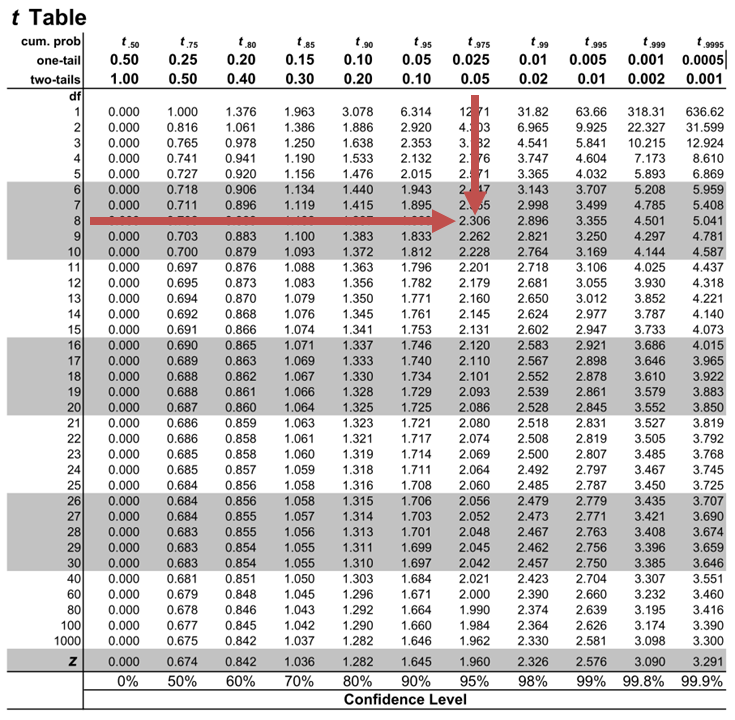
Notice that \(|t|>t_{c}\) i.e., (\(10.85>2.306\))

Therefore, we reject the null hypothesis and conclude that the estimated slope coefficient is statistically different from one.

Note that we used the confidence interval approach and arrived at the same conclusion.

Question Neeth Shinu, CFA, is forecasting price elasticity of supply for a certain product. Shinu uses the quantity of the product supplied for the past 5months as the dependent variable and the price per unit of the product as the independent variable. The regression results are shown below. $$\small{\begin{array}{lccccc}\hline \textbf{Regression Statistics} & & & & & \\ \hline \text{Multiple R} & 0.9971 & {}& {}&{}\\ \text{R Square} & 0.9941 & & & \\ \text{Adjusted R Square} & 0.9922 & & & & \\ \text{Standard Error} & 3.6515 & & & \\ \text{Observations} & 5 & & & \\ \hline {}& \textbf{Coefficients} & \textbf{Standard Error} & \textbf{t Stat} & \textbf{P-value}\\ \hline\text{Intercept} & -159 & 10.520 & (15.114) & 0.001\\ \text{Slope} & 0.26 & 0.012 & 22.517 & 0.000\\ \hline\end{array}}$$ Which of the following most likely reports the correct value of the t-statistic for the slope and most accurately evaluates its statistical significance with 95% confidence?     A. \(t=21.67\); slope is significantly different from zero.     B. \(t= 3.18\); slope is significantly different from zero.     C. \(t=22.57\); slope is not significantly different from zero. Solution The correct answer is A . The t-statistic is calculated using the formula: $$\text{t}=\frac{\widehat{b_{1}}-b_1}{\widehat{S_{b_{1}}}}$$ Where: \(b_{1}\) = True slope coefficient \(\widehat{b_{1}}\) = Point estimator for \(b_{1}\) \(\widehat{S_{b_{1}}}\) = Standard error of the regression coefficient $$\begin{align*}\text{t}&=\frac{0.26-0}{0.012}\\&=21.67\end{align*}$$ The critical two-tail t-values from the t-table with \(n-2 = 3\) degrees of freedom are: $$t_{c}=±3.18$$ Notice that \(|t|>t_{c}\) (i.e \(21.67>3.18\)). Therefore, the null hypothesis can be rejected. Further, we can conclude that the estimated slope coefficient is statistically different from zero.

Offered by AnalystPrep

Analysis of Variance (ANOVA)

Predicted value of a dependent variable, understanding the decision rule.

The decision rule refers to the procedure followed by analysts and researchers when... Read More

Functional Forms for Simple Linear Reg ...

To address non-linear relationships, we employ various functional forms to potentially convert the... Read More

Cash Flow Additivity

A timeline is a physical illustration of the amounts and timing of cashflows... Read More

Downside Deviation

When trying to estimate downside risk (i.e., returns below the mean), we can... Read More

Encyclopedia of Quality of Life and Well-Being Research pp 3569–3571 Cite as

Intercept, Slope in Regression

• Melanie Revilla 2  
• Reference work entry
• First Online: 01 January 2024

The slope is the increase in the dependent variable when the independent variable increases with one unit and all other independent variables remain the same.

The intercept is the value of the dependent variables if all independent variables have the value zero.

Description

In statistics, the term “regression analyses” is used to refer to any techniques of analysis of the data focusing on the relationship between a dependent variable and one or more independent variables (Montgomery et al. 2001 ). The dependent variable is also called endogenous variable and is by convention usually denoted by the capital letter Y. It is the variable of interest. The independent variables are also called exogenous variables and are by convention usually denoted by the capital letter X. When several independent variables are introduced in the model, the indices i are used to distinguish them: X i is the i th independent variable. The independent variables are the ones that we believe can...

This is a preview of subscription content, log in via an institution .

Buying options

• Available as PDF
• Read on any device
• Instant download
• Own it forever
• Available as EPUB and PDF
• Durable hardcover edition
• Dispatched in 3 to 5 business days
• Free shipping worldwide - see info

Tax calculation will be finalised at checkout

Purchases are for personal use only

Montgomery, D. C., Peck, E. A., & Vining, G. G. (2001). Introduction to linear regression analysis . Hoboken: Wiley.

Google Scholar  

Download references

Author information

Authors and affiliations.

Political and Social Sciences, Universitat Pompeu Fabra RECSM, Barcelona, Spain

Melanie Revilla

You can also search for this author in PubMed   Google Scholar

Corresponding author

Correspondence to Melanie Revilla .

Editor information

Editors and affiliations.

Dipartimento di Scienze Statistiche, Sapienza Università di Roma, Roma, Roma, Italy

Filomena Maggino

Section Editor information

Department of Political Science, University of Naples Federico II, Naples, Italy

Mara Tognetti

Rights and permissions

Reprints and permissions

Copyright information

© 2023 Springer Nature Switzerland AG

About this entry

Cite this entry.

Revilla, M. (2023). Intercept, Slope in Regression. In: Maggino, F. (eds) Encyclopedia of Quality of Life and Well-Being Research. Springer, Cham. https://doi.org/10.1007/978-3-031-17299-1_1486

Download citation

DOI : https://doi.org/10.1007/978-3-031-17299-1_1486

Published : 11 February 2024

Publisher Name : Springer, Cham

Print ISBN : 978-3-031-17298-4

Online ISBN : 978-3-031-17299-1

eBook Packages : Social Sciences Reference Module Humanities and Social Sciences Reference Module Business, Economics and Social Sciences

Share this entry

Anyone you share the following link with will be able to read this content:

Sorry, a shareable link is not currently available for this article.

Provided by the Springer Nature SharedIt content-sharing initiative

• Publish with us

Policies and ethics

• Find a journal
• Track your research

Hypothesis Tests on Slope Coefficient

Understanding hypothesis testing for linear regression | cfa level i quantitative methods.

In our last lesson, we ended off by learning how to calculate the confidence interval of a forecast made by our linear regression model. Besides the uncertainty of the forecast, there are other uncertainties of the estimates that are of interest, like the intercept and slope coefficient. In this lesson, we apply the statistical tools on the slope coefficient, but the same tools can be applied on the intercept as well.

Setting up Hypothesis Testing for Slope Coefficient

Let’s say you believe that there is a relationship between the company profit and the bonus payouts. Your alternate hypothesis (H a ) should be that the slope coefficient b1 ≠0. This is because if there is a relationship, the slope coefficient should be significantly different from zero. Your null hypothesis (H0) should therefore be b1=0, which implies there is no relationship between the company profits and bonus.

Using Confidence Interval for Hypothesis Testing

Calculating the 95% Confidence Interval for the Slope Coefficient Estimate:

Step 1: Point Estimate

The point estimate is simply the slope coefficient, which we estimate as 0.3.

Step 2: Critical Value

We use the t-statistic here, with a degree of freedom of n-2 as there are two estimated parameters in a simple linear regression. With 2 degrees of freedom and a two-tailed significance level of 5%, we get a critical value of 4.303.

Step 3: Standard Error

Let’s say we are told that the standard error for the coefficient is 0.18.

Step 4: Calculating the 95% Confidence Interval

Plugging in all the figures into the confidence interval formula, we get an interval of between -0.47 and 1.07.

Lower Bound: 0.3 – (4.303 × 0.18) = -0.47

Upper Bound: 0.3 + (4.303 × 0.18) = 1.07

Since zero falls within the confidence interval , we are unable to reject the null hypothesis . This means that at the 95% confidence level, there is insufficient evidence to support your hypothesis that there is a linear relationship between company profit and bonus payouts.

Using t-test for Hypothesis Testing

Another approach is to simply use a t-test, whereby we calculate the t-statistic , which is to measure how many standard deviations our estimate is away from the hypothesized value. In our example, we get a t-statistic = (0.3 / 0.18) = 1.667.

Since our t-statistic (1.667) is not within the rejection region ( critical value of 4.303), we fail to reject the null hypothesis . We cannot conclude that there is a positive relationship between company profits and the number of months bonus at the 5% significance level .

Hypothesis Testing with TinyPower Example

p-value and Hypothesis Testing

In hypothesis testing, the choice of significance level is always a matter of judgment. If we use a higher significance level , we may be able to reject the null hypothesis . However, that also increases the probability of a Type 1 error, which is the probability of rejecting the null hypothesis when it is actually true. On the flip side, if we use a significance that is too low, the probability of a Type 2 error increases, that is failing to reject the null hypothesis when it is actually false.

So rather than reporting whether a particular hypothesis is rejected or not, some analysts prefer to report the p-value or probability value for the reader to interpret the results. The p-value is the smallest level of significance at which the null hypothesis can be rejected . In our example, the t-statistic 1.667 we calculated earlier falls somewhere between probabilities of 0.2 and 0.3 on the t-table, so the p-value is around 0.24. This means that we can reject the null hypothesis at around the 24% significance level . This figure allows the reader to form his own opinion with regards to the hypothesis. As in this case, the reader may find that the p-value is too high, so he may disregard the findings of the hypothesis.

Understanding the F-Test in Linear Regression

In this lesson, we will explore the F-test in linear regression analysis and discuss some limitations of regression analysis . The F-test is used to determine if there is a significant relationship between the independent and dependent variables in a linear regression model.

F-Test and the ANOVA Table

First, let’s recap the ANOVA table from our previous lesson. The table consists of explained and unexplained variation:

• Explained variation ( Regression Sum of Squares – RSS ): The portion of the total variation that is explained by the regression model.
• Unexplained variation ( Sum of Squared Errors – SSE ): The portion of the total variation that remains unexplained by the regression model.

The F-statistic is calculated as follows:

F-statistic = Mean Square Regression ( MSR ) / Mean Square Error ( MSE )

A high F-statistic indicates that the linear regression is a good fit, suggesting a significant relationship between the independent and dependent variables.

Given an ANOVA table with the following values: n = 4, SSE = 0.86, RSS = 6.9. Calculate the F-statistic and determine if there is a significant relationship between the dependent and independent variables at a 5% level of significance .

Calculate the degrees of freedom (DF) for explained and unexplained variation: DF1 (explained) = 1, DF2 (unexplained) = N – 2 = 4 – 2 = 2

Calculate the MSR and MSE : MSR = RSS / DF1 = 6.9 / 1 = 6.9 MSE = SSE / DF2 = 0.86 / 2 = 0.43

Calculate the F-statistic : F-statistic = MSR / MSE = 6.9 / 0.43 = 16.05

To determine if the F-statistic is significant, we compare it to the critical value from the F-table: Find the critical value for a 5% level of significance with DF1 = 1 and DF2 = 2. The critical value is 18.5. Since 16.05 < 18.5, we cannot reject the null hypothesis . There is no significant relationship between the dependent and independent variables at the 5% level of significance .

✨ Visual Learning Unleashed! ✨ [Premium]

Elevate your learning with our captivating animation video—exclusive to Premium members! Watch this lesson in much more detail with vivid visuals that enhance understanding and make lessons truly come alive. 🎬

Unlock the power of visual learning—upgrade to Premium and click the link NOW! 🌟

• Term: Regression sum of squares
• Term: Level of significance
• Term: Sum of squared errors
• Term: Independent variable
• Term: Regression analysis
• Term: Confidence interval
• Term: Null hypothesis
• Term: Point estimate
• Term: Critical value
• Term: ANOVA table
• Term: F-statistic
• Term: t-statistic
• Term: F-test
• Term: Mean regression sum of squares
• Term: Mean squared error

[fvplayer id=”3″]

This refund processing fee is to compensate us for the payment processing fee that we paid when you made the purchase.

Have you ever gotten stuck in your study because you can’t remember a formula, or what a specific term means? Now, say goodbye to scanning through all the videos and ploughing through pages and pages just to find what you are looking for. All the important formulas, definitions and diagrams you need for the exam are now at your fingertips at prepnuggets.com/glossary .

What’s more, these quick references are deeply integrated in our lessons, so you get a good idea of what the lesson covers even before watching the video. The references also point you to specific video lessons where it is covered, so you can quickly access the corresponding video to learn more about the term.

Available now for all Level I topics ,  this service is exclusive for our Premium and Pro members only. We will progressively add the rest of the topic areas over the next few months.

We think this is a game-changer for your CFA success!

Hey visitor,

Are you a CFA Level I candidate, or someone who is exploring taking the CFA exam? Four years ago, I was in your shoes. I am a Computer Engineering graduate and have been working as an engineer all my life. Having developed a keen interest in finance, I decided on a career switch to the finance field and enrolled into the CFA program at the same time.

Was it tough? You bet!

Adjusting to the drastic career change was tough. I naturally neglected the preparation for my Level I exam in June 2014. It was not until the middle of March 2014 that I realized I only had a little more than 2 months to the exam. To compound my problems, I basically did not have a preparation strategy. Having no background in finance at all, I tried very hard to read the curriculum from cover to cover, but eventually that fell flat. I can still recall the number of times I dozed off while studying, or just going back and forth trying to understand even the simplest concept. My mind simply could not keep up after a hard day at work.

Does all these sound familiar to you? Well, take heart. No matter how bleak it seems, at least sit for the exam and treat it as a learning experience. That was basically my attitude as I burrowed through my exam prep with toil and stress. By God’s grace, I did pass my Level I exam in June 2014. It was an experience I would not want to revisit though.

Tweaking the approach

For the Level II exam, I endeavoured not to repeat the mistakes I made. Based on the Pareto 80/20 principle, I learnt to extract the most essential bits from the curriculum enough to give me that 80% result to pass. Being a visual learner, I took notes and summaries in pictorial form. Instead of reserving huge segments of time to study, I carved out pockets of time to learn and practise – accommodating to my full-time job. I managed to pass my Level II and Level III exams consecutively with considerably less effort and stress than when I did my level I.

Why PrepNuggets?

I love the CFA Program and truly value the skills and ethics that are imparted to make me a better finance professional. My desire is to help candidates who are keen to pursue this path to do so in the most effective and painless process as possible – based on the lessons that I learnt as a candidate. I have set up PrepNuggets with the vision to revolutionise learning by using technology, catering to the short attention span that we can afford. If this makes sense to you, join the PrepNuggets community by signing up for your free student account. I am confident that the materials that we have laboriously crafted will bring you closer to that dream pass with just that 20% effort. Let us do the hard work for you.

Keith Tan, CFA Founder and Chief Instructor PrepNuggets

About the Author

PrepNuggets

Keith is the founder and chief instructor of PrepNuggets. He has a wide range of interests in all things related to tech, from web development to e-learning, gadgets to apps. Keith loves exploring different cultures and the untouched gems around the world. He currently lives in Singapore but frequently travels to share his knowledge and expertise with others.

Username or Email Address

Remember Me

• 3.6 - Further SLR Evaluation Examples

Example 1: Are Sprinters Getting Faster?

The following data set ( mens200m.txt ) contains the winning times (in seconds) of the 22 men's 200 meter olympic sprints held between 1900 and 1996. (Notice that the Olympics were not held during the World War I and II years.) Is there a linear relationship between year and the winning times? The plot of the estimated regression line sure makes it look so!

To answer the research question, let's conduct the formal F -test of the null hypothesis H 0 : β 1 = 0 against the alternative hypothesis H A : β 1 ≠ 0.

The analysis of variance table above has been animated to allow you to interact with the table. As you roll your mouse over the blue numbers , you are reminded of how those numbers are determined.

From a scientific point of view, what we ultimately care about is the P -value, which is 0.000 (to three decimal places). That is, the P -value is less than 0.001. The P -value is very small. It is unlikely that we would have obtained such a large F* statistic if the null hypothesis were true. Therefore, we reject the null hypothesis H 0 : β 1 = 0 in favor of the alternative hypothesis H A : β 1 ≠ 0. There is sufficient evidence at the α = 0.05 level to conclude that there is a linear relationship between year and winning time.

Equivalence of the analysis of variance F -test and the t -test

As we noted in the first two examples, the P -value associated with the t -test is the same as the P -value associated with the analysis of variance F -test. This will always be true for the simple linear regression model. It is illustrated in the year and winning time example also. Both P -values are 0.000 (to three decimal places):

The P -values are the same because of a well-known relationship between a t random variable and an F random variable that has 1 numerator degree of freedom. Namely:

\[(t^{*}_{(n-2)})^2=F^{*}_{(1,n-2)}\]

This will always hold for the simple linear regression model. This relationship is demonstrated in this example as:

(-13.33) 2 = 177.7

• For a given significance level α, the F -test of β 1 = 0 versus β 1 ≠ 0 is algebraically equivalent to the two-tailed t -test.
• If one test rejects H 0 , then so will the other.
• If one test does not reject H 0 , then so will the other.

The natural question then is ... when should we use the F -test and when should we use the t -test?

• The F -test is only appropriate for testing that the slope differs from 0 ( β 1 ≠ 0).
• Use the t -test to test that the slope is positive ( β 1 > 0) or negative ( β 1 < 0). Remember, though, that you will have to divide the reported two-tail P -value by 2 to get the appropriate one-tailed P -value.

The F -test is more useful for the multiple regression model when we want to test that more than one slope parameter is 0. We'll learn more about this later in the course!

Example 2: Highway Sign Reading Distance and Driver Age

The data are n = 30 observations on driver age and the maximum distance (feet) at which individuals can read a highway sign ( signdist.txt ). (Data source: Mind On Statistics , 3rd edition, Utts and Heckard).

The plot below gives a scatterplot of the highway sign data along with the least squares regression line. 

Here is the accompanying regression output:

Hypothesis Test for the Intercept ( β 0 )

This test is rarely a test of interest, but does show up when one is interested in performing a regression through the origin (which we touched on earlier in this lesson). In the software output above, the row labeled Constant gives the information used to make inferences about the intercept. The null and alternative hypotheses for a hypotheses test about the intercept are written as:

H 0 : β 0 = 0 H A :  β 0 ≠ 0.

In other words, the null hypothesis is testing if the population intercept is equal to 0 versus the alternative hypothesis that the population intercept is not equal to 0. In most problems, we are not particularly interested in hypotheses about the intercept. For instance, in our example, the intercept is the mean distance when the age is 0, a meaningless age. Also, the intercept does not give information about how the value of y changes when the value of x changes. Nevertheless, to test whether the population intercept is 0, the information from the software output would be used as follows:

• The sample intercept is b 0 = 576.68, the value under Coef .
• The standard error (SE) of the sample intercept, written as se( b 0 ), is se( b 0 ) = 23.47, the value under SE Coef. The SE of any statistic is a measure of its accuracy. In this case, the SE of b 0 gives, very roughly, the average difference between the sample b 0 and the true population intercept  β 0 , for random samples of this size (and with these x -values).
• The test statistic is t = b 0 /se( b 0 ) = 576.68/23.47 = 24.57, the value under T.
• The p -value for the test is p = 0.000 and is given under P. The p -value is actually very small and not exactly 0.
• The decision rule at the 0.05 significance level is to reject the null hypothesis since our p < 0.05. Thus, we conclude that there is statistically significant evidence that the population intercept is not equal to 0.

So how exactly is the p -value found? For simple regression, the p -value is determined using a t distribution with n − 2 degrees of freedom ( df ), which is written as t n −2 , and is calculated as 2 × area past | t | under a t n −2 curve. In this example, df = 30 − 2 = 28. The p -value region is the type of region shown in the figure below. The negative and positive versions of the calculated t provide the interior boundaries of the two shaded regions. As the value of t increases, the p -value (area in the shaded regions) decreases.

Hypothesis Test for the Slope ( β 1 )

This test can be used to test whether or not x and y are linearly related. The row pertaining to the variable Age in the software output from earlier gives information used to make inferences about the slope. The slope directly tells us about the link between the mean y and x . When the true population slope does not equal 0, the variables y and x are linearly related. When the slope is 0, there is not a linear relationship because the mean y does not change when the value of x is  changed. The null and alternative hypotheses for a hypotheses test about the slope are written as:

H 0 : β 1 = 0 H A : β 1 ≠ 0.

In other words, the null hypothesis is testing if the population slope is equal to 0 versus the alternative hypothesis that the population slope is not equal to 0. To test whether the population slope is 0, the information from the software output is used as follows:

• The sample slope is b 1 = −3.0068, the value under Coef in the Age row of the output.
• The SE of the sample slope, written as se( b 1 ), is se( b 1 ) = 0.4243, the value under SE Coef . Again, the SE of any statistic is a measure of its accuracy. In this case, the SE of b1 gives, very roughly, the average difference between the sample b 1 and the true population slope  β 1 , for random samples of this size (and with these x -values).
• The test statistic is t = b 1 /se( b 1 ) = −3.0068/0.4243 = −7.09, the value under T.
• The p -value for the test is p = 0.000 and is given under P.
• The decision rule at the 0.05 significance level is to reject the null hypothesis since our p < 0.05. Thus, we conclude that there is statistically significant evidence that the variables of Distance and Age are linearly related.

As before, the p -value is the region illustrated in the figure above.

Confidence Interval for the Slope ( β 1 )

A confidence interval for the unknown value of the population slope β 1 can be computed as

sample statistic ± multiplier × standard error of statistic

→ b 1 ± t * × se( b 1 ).

In simple regression, the t * multiplier is determined using a t n −2 distribution. The value of t * is such that the confidence level is the area (probability) between − t * and + t * under the t -curve. To find the t * multiplier, you can do one of the following:

• A table such as the one in the textbook can be used to look up the multiplier.
• Alternatively, software like Minitab can be used.

95% Confidence Interval

In our example, n = 30 and df = n − 2 = 28. For 95% confidence, t * = 2.05. A 95% confidence interval for β 1 , the true population slope, is:

−3.0068 ± (2.05 × 0.4243) −3.0068 ± 0.870 or about − 3.88 to − 2.14.

Interpretation: With 95% confidence, we can say the mean sign reading distance decreases somewhere between 2.14 and 3.88 feet per each one-year increase in age. It is incorrect to say that with 95% probability the mean sign reading distance decreases somewhere between 2.14 and 3.88 feet per each one-year increase in age. Make sure you understand why!!!

99% Confidence Interval

For 99% confidence, t * = 2.76. A 99% confidence interval for β 1 , the true population slope is:

−3.0068 ± (2.76 × 0.4243) −3.0068 ± 1.1711 or about − 4.18 to − 1.84.

Interpretation: With 99% confidence, we can say the mean sign reading distance decreases somewhere between 1.84 and 4.18 feet per each one-year increase in age. Notice that as we increase our confidence, the interval becomes wider. So as we approach 100% confidence, our interval grows to become the whole real line.

As a final note, the above procedures can be used to calculate a confidence interval for the population intercept. Just use b 0 (and its standard error) rather than b 1 .

Example 3: Handspans Data

Stretched handspans and heights are measured in centimeters for n = 167 college students ( handheight.txt ). We’ll use y = height and x = stretched handspan. A scatterplot with a regression line superimposed is given below, together with results of a simple linear regression model fit to the data.

Some things to note are:

• The residual standard deviation S is 2.744 and this estimates the standard deviation of the errors.
• r 2 = (SSTO-SSE) / SSTO = SSR / (SSR+SSE) = 1500.1 / (1500.1+1242.7) = 1500.1 / 2742.8 = 0.547 or 54.7%. The interpretation is that handspan differences explain 54.7% of the variation in heights.
• The value of the F statistic is F = 199.2 with 1 and 165 degrees of freedom, and the p -value for this F statistic is 0.000. Thus we reject the null hypothesis H 0 : β 1 = 0 because the p -value is so small. In other words, the observed relationship is statistically significant.

Start Here!

• Welcome to STAT 462!
• Search Course Materials
• Lesson 1: Statistical Inference Foundations
• Lesson 2: Simple Linear Regression (SLR) Model
• 3.1 - Inference for the Population Intercept and Slope
• 3.2 - Another Example of Slope Inference
• 3.3 - Sums of Squares
• 3.4 - Analysis of Variance: The Basic Idea
• 3.5 - The Analysis of Variance (ANOVA) table and the F-test
• 3.7 - Decomposing The Error When There Are Replicates
• 3.8 - The Lack of Fit F-test When There Are Replicates
• Lesson 4: SLR Assumptions, Estimation & Prediction
• Lesson 5: Multiple Linear Regression (MLR) Model & Evaluation
• Lesson 6: MLR Assumptions, Estimation & Prediction
• Lesson 7: Transformations & Interactions
• Lesson 8: Categorical Predictors
• Lesson 9: Influential Points
• Lesson 10: Regression Pitfalls
• Lesson 11: Model Building
• Lesson 12: Logistic, Poisson & Nonlinear Regression
• Website for Applied Regression Modeling, 2nd edition
• Notation Used in this Course
• R Software Help
• Minitab Software Help

Copyright © 2018 The Pennsylvania State University Privacy and Legal Statements Contact the Department of Statistics Online Programs

Do you get more food when you order in-person at Chipotle?

April 7, 2024

Inspired by this Reddit post , we will conduct a hypothesis test to determine if there is a difference in the weight of Chipotle orders between in-person and online orders. The data was originally collected by Zackary Smigel , and a cleaned copy be found in data/chipotle.csv .

Throughout the application exercise we will use the infer package which is part of tidymodels to conduct our permutation tests.

Variable type: character

Variable type: Date

Variable type: numeric

The variable we will use in this analysis is weight which records the total weight of the meal in grams.

We wish to test the claim that the difference in weight between in-person and online orders must be due to something other than chance.

• Your turn: Write out the correct null and alternative hypothesis in terms of the difference in means between in-person and online orders. Do this in both words and in proper notation.

Null hypothesis: TODO

\[H_0: \mu_{\text{online}} - \mu_{\text{in-person}} = TODO\]

Alternative hypothesis: The difference in means between in-person and online Chipotle orders is not \(0\) .

\[H_A: \mu_{\text{online}} - \mu_{\text{in-person}} TODO\]

Observed data

Our goal is to use the collected data and calculate the probability of a sample statistic at least as extreme as the one observed in our data if in fact the null hypothesis is true.

• Demo: Calculate and report the sample statistic below using proper notation.

The null distribution

Let’s use permutation-based methods to conduct the hypothesis test specified above.

We’ll start by generating the null distribution.

• Demo: Generate the null distribution.
• Your turn: Take a look at null_dist . What does each element in this distribution represent?

Add response here.

Question: Before you visualize the distribution of null_dist – at what value would you expect this distribution to be centered? Why?

Demo: Create an appropriate visualization for your null distribution. Does the center of the distribution match what you guessed in the previous question?

• Demo: Now, add a vertical red line on your null distribution that represents your sample statistic.

Question: Based on the position of this line, does your observed sample difference in means appear to be an unusual observation under the assumption of the null hypothesis?

Above, we eyeballed how likely/unlikely our observed mean is. Now, let’s actually quantify it using a p-value.

Question: What is a p-value?

Guesstimate the p-value

• Demo: Visualize the p-value.

Your turn: What is you guesstimate of the p-value?

Calculate the p-value

Your turn: What is the conclusion of the hypothesis test based on the p-value you calculated? Make sure to frame it in context of the data and the research question. Use a significance level of 5% to make your conclusion.

Demo: Interpret the p-value in context of the data and the research question.

Reframe as a linear regression model

While we originally evaluated the null/alternative hypotheses as a difference in means, we could also frame this as a regression problem where the outcome of interest (weight of the order) is a continuous variable. Framing it this way allows us to include additional explanatory variables in our model which may account for some of the variation in weight.

Single explanatory variable

Demo: Let’s reevaluate the original hypotheses using a linear regression model. Notice the similarities and differences in the code compared to a difference in means, and that the obtained p-value should be nearly identical to the results from the difference in means test.

Multiple explanatory variables

Demo: Now let’s also account for additional variables that likely influence the weight of the order.

• Protein type ( meat )
• Type of meal ( meal_type ) - burrito or bowl
• Store ( store ) - at which Chipotle location the order was placed

Your turn: Interpret the p-value for the order in context of the data and the research question.

Compare to CLT-based method

Demo: Let’s compare the p-value obtained from the permutation test to the p-value obtained from that derived using the Central Limit Theorem (CLT).

Your turn: What is the p-value obtained from the CLT-based method? How does it compare to the p-value obtained from the permutation test?