discussion of findings in research pdf

When you choose to publish with PLOS, your research makes an impact. Make your work accessible to all, without restrictions, and accelerate scientific discovery with options like preprints and published peer review that make your work more Open.

• PLOS Biology
• PLOS Climate
• PLOS Complex Systems
• PLOS Computational Biology
• PLOS Digital Health
• PLOS Genetics
• PLOS Global Public Health
• PLOS Medicine
• PLOS Mental Health
• PLOS Neglected Tropical Diseases
• PLOS Pathogens
• PLOS Sustainability and Transformation
• PLOS Collections
• How to Write Discussions and Conclusions

The discussion section contains the results and outcomes of a study. An effective discussion informs readers what can be learned from your experiment and provides context for the results.

What makes an effective discussion?

When you’re ready to write your discussion, you’ve already introduced the purpose of your study and provided an in-depth description of the methodology. The discussion informs readers about the larger implications of your study based on the results. Highlighting these implications while not overstating the findings can be challenging, especially when you’re submitting to a journal that selects articles based on novelty or potential impact. Regardless of what journal you are submitting to, the discussion section always serves the same purpose: concluding what your study results actually mean.

A successful discussion section puts your findings in context. It should include:

• the results of your research,
• a discussion of related research, and
• a comparison between your results and initial hypothesis.

Tip: Not all journals share the same naming conventions.

You can apply the advice in this article to the conclusion, results or discussion sections of your manuscript.

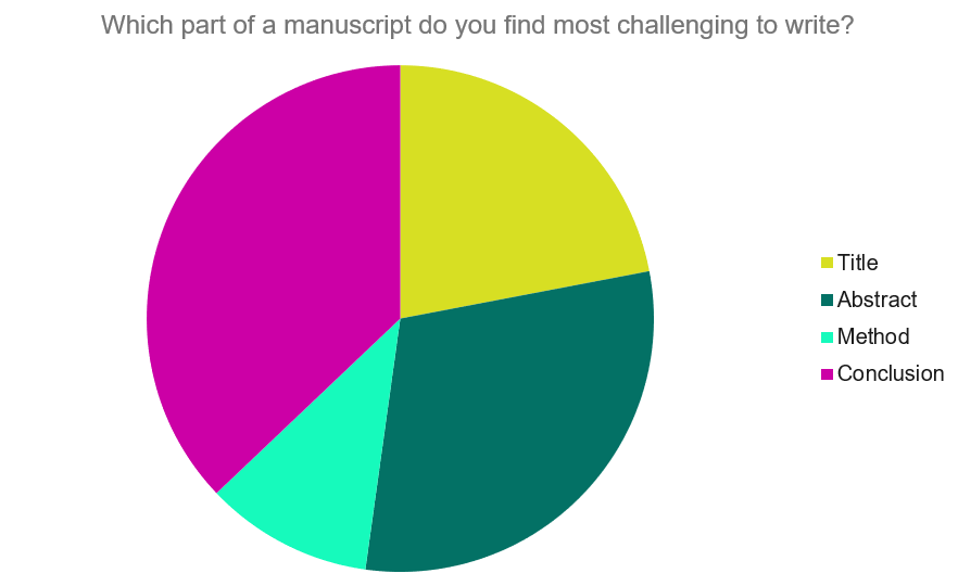
Our Early Career Researcher community tells us that the conclusion is often considered the most difficult aspect of a manuscript to write. To help, this guide provides questions to ask yourself, a basic structure to model your discussion off of and examples from published manuscripts. 

Questions to ask yourself:

• Was my hypothesis correct?
• If my hypothesis is partially correct or entirely different, what can be learned from the results? 
• How do the conclusions reshape or add onto the existing knowledge in the field? What does previous research say about the topic? 
• Why are the results important or relevant to your audience? Do they add further evidence to a scientific consensus or disprove prior studies? 
• How can future research build on these observations? What are the key experiments that must be done? 
• What is the “take-home” message you want your reader to leave with?

How to structure a discussion

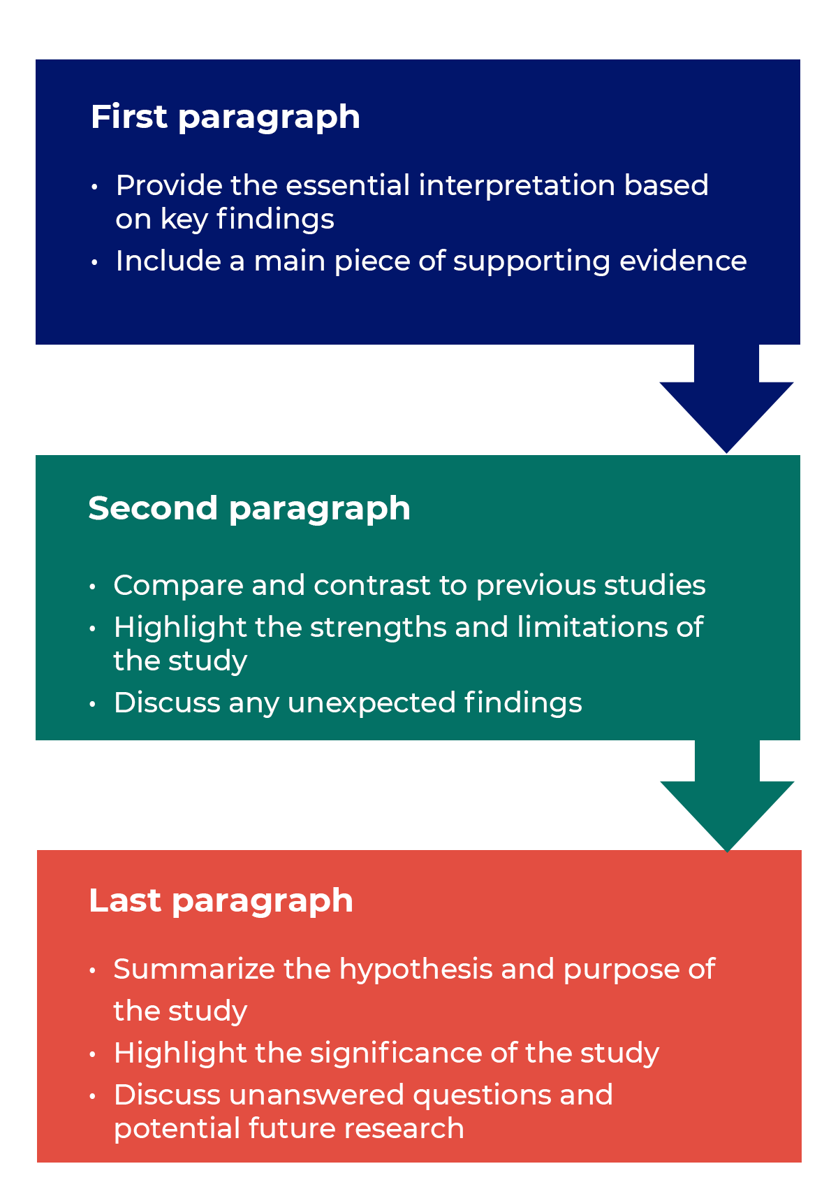
Trying to fit a complete discussion into a single paragraph can add unnecessary stress to the writing process. If possible, you’ll want to give yourself two or three paragraphs to give the reader a comprehensive understanding of your study as a whole. Here’s one way to structure an effective discussion:

Writing Tips

While the above sections can help you brainstorm and structure your discussion, there are many common mistakes that writers revert to when having difficulties with their paper. Writing a discussion can be a delicate balance between summarizing your results, providing proper context for your research and avoiding introducing new information. Remember that your paper should be both confident and honest about the results! 

• Read the journal’s guidelines on the discussion and conclusion sections. If possible, learn about the guidelines before writing the discussion to ensure you’re writing to meet their expectations. 
• Begin with a clear statement of the principal findings. This will reinforce the main take-away for the reader and set up the rest of the discussion. 
• Explain why the outcomes of your study are important to the reader. Discuss the implications of your findings realistically based on previous literature, highlighting both the strengths and limitations of the research. 
• State whether the results prove or disprove your hypothesis. If your hypothesis was disproved, what might be the reasons? 
• Introduce new or expanded ways to think about the research question. Indicate what next steps can be taken to further pursue any unresolved questions. 
• If dealing with a contemporary or ongoing problem, such as climate change, discuss possible consequences if the problem is avoided. 
• Be concise. Adding unnecessary detail can distract from the main findings. 

Don’t

• Rewrite your abstract. Statements with “we investigated” or “we studied” generally do not belong in the discussion. 
• Include new arguments or evidence not previously discussed. Necessary information and evidence should be introduced in the main body of the paper. 
• Apologize. Even if your research contains significant limitations, don’t undermine your authority by including statements that doubt your methodology or execution. 
• Shy away from speaking on limitations or negative results. Including limitations and negative results will give readers a complete understanding of the presented research. Potential limitations include sources of potential bias, threats to internal or external validity, barriers to implementing an intervention and other issues inherent to the study design. 
• Overstate the importance of your findings. Making grand statements about how a study will fully resolve large questions can lead readers to doubt the success of the research. 

Snippets of Effective Discussions:

Consumer-based actions to reduce plastic pollution in rivers: A multi-criteria decision analysis approach

Identifying reliable indicators of fitness in polar bears

• How to Write a Great Title
• How to Write an Abstract
• How to Write Your Methods
• How to Report Statistics
• How to Edit Your Work

The contents of the Peer Review Center are also available as a live, interactive training session, complete with slides, talking points, and activities. …

The contents of the Writing Center are also available as a live, interactive training session, complete with slides, talking points, and activities. …

There’s a lot to consider when deciding where to submit your work. Learn how to choose a journal that will help your study reach its audience, while reflecting your values as a researcher…

Mastering Your Dissertation pp 105–115 Cite as

How Do I Write the Discussion Chapter?

Reflecting on and Comparing Your Data, Recognising the Strengths and Limitations

• Sue Reeves   ORCID: orcid.org/0000-0002-3017-0559 3 &
• Bartek Buczkowski   ORCID: orcid.org/0000-0002-4146-3664 4  
• First Online: 19 October 2023

316 Accesses

The Discussion chapter brings an opportunity to write an academic argument that contains a detailed critical evaluation and analysis of your research findings. This chapter addresses the purpose and critical nature of the discussion, contains a guide to selecting key results to discuss, and details how best to structure the discussion with subsections and paragraphs. We also present a list of points to do and avoid when writing the discussion together with a Discussion chapter checklist.

Download chapter PDF

9.1 Introduction

Arguably, the Discussion chapter is the most interesting and most important chapter in any dissertation or thesis. Discussing the results should feel exciting to you because this is where the story of your dissertation should at last become clear. The discussion is so much more than just a comparison of your results to those published in previous studies conducted in your area of research. The discussion is a place for rich reflection on the research journey that you undertook. As the discussion is one of the most critical chapters in any dissertation or thesis, reference will be made to critical skills throughout this chapter.

9.2 What Is the Discussion Chapter?

What does it mean to “discuss” the results? In the world of academia, we discuss research continuously, we argue a point, and we are expected to build a case or an “academic argument”. Note that “arguing” in academic terms does not refer to shouting or gesturing but simply to presenting evidence (or reasoning) why we think that something is important, meaningful, contributes new knowledge, corroborates points made earlier, or contradicts points previously made. We need to pay attention to detail, and to do so requires an open mind, since in the discussion you may have to confront hard facts and evidence and put aside any ideas that you may have previously had about your research topic. You should, therefore, interrogate the meaning of your results. There are elements of reflection in the discussion chapter, and this reflection pertains to the impact of the decisions that were made at the planning stage of the research and data collection (such as choice of methods for data collection) on the outcomes of the research.

To put it simply, the Discussion chapter, is where you critically appraise your own study. At this stage, critical appraisal should be familiar to you. You have critically appraised literature in the Introduction and Literature Review chapter. You critically appraised methods that were used in previous studies, and you justified the choice of methods in the Methodology chapter. In the Discussion chapter you are expected to analyse and appraise the findings of your data analysis.

McGregor ( 2018 ) points out the threefold purpose of the Discussion chapter:

To summarise salient findings.

To explain the findings.

To analyse the implications of the findings.

Salient findings are those that are the most important, i.e. the key findings from your data analysis. We will come back to the term “key results” later in this chapter.

9.3 What Should the Discussion Chapter Look like?

Every chapter that you have written so far has a base of some sort. The literature review is the theoretical base for your research project. Based on previous research, you built an argument that details why your research is worth performing, you may have identified gaps in knowledge, and you constructed an aim, objectives, and hypotheses. You defined your research idea with clear reference to previously undertaken and published research. You used the literature base to define methods that allowed you to collect data, the analysis of which would allow you to address your research aim. This is a rather long way to say that the Discussion chapter is the place in your dissertation where you draw on all of the above elements—the literature base, the methods that you used, and your results.

The discussion should be structured in such a way that it allows you to place your results in the context of a bigger body of research. This means that you interpret your results (“what do the results mean?”) and explain them with reference to results from other similar studies (compare but also provide an explanation of things that could have affected the results). You should also consider the strengths and limitations of your approach and explain the implications of your results (the “so what?”) to put them in context.

The fact that you are required to evaluate your research with reference to previous studies means that you will need to include references but be careful—avoid writing a discussion that reads like Literature Review version 2.0.

The discussion is a gateway to the next chapter—the Conclusion, and a well-thought through, and thorough critical discussion of the results that you collected in the course of your research project will make the writing of the conclusion a lot easier.

9.4 Do I Discuss all my Results?

Not every single result has to be discussed. Remember that criticality in academic writing is demonstrated in a multitude of ways. We sometimes fall into the trap of “compare and contrast” our findings with those of other authors as the only way to demonstrate criticality. However, being selective in academic writing is also a mark of criticality. This selectivity means choosing the key results to discuss and treating these key results with meticulous attention to detail. The more of your results you try to squeeze into the Discussion, the more superficial and diluted this chapter could appear. Hence, the discussion chapter should contain a detailed discussion of key results, with an acknowledgement of less important results.

9.5 How Do I Decide which Results Are Key?

In the previous chapter, we explored statistical significance. Some students use “statistically significant” results as the “key results”. However, please be mindful that key results are those results that align with the research question that you set out to explore and relate to your aims and objectives. Logic dictates that these results do not necessarily have to be statistically significant at p ≤ 0.05. Sometimes lack of statistical significance in a set of results is also a really telling finding.

Earlier in this chapter, we remarked upon the multitude of activities that you undertook in your research project to arrive at this stage—to be able to critically analyse and interpret your results. You should have a good insight into which of the results allow you to address the research question. Consult with your supervisor and use your judgement as to which results from your data analysis are the key results.

Cottrell (2017) points out that critical writers are aware of their audience (readership). A good way to decide which are the key results of your research project is by asking yourself “what do I want my readers to get out of my project?” Additionally, if you are a postgraduate research student and you are required to take your thesis to a viva voce, you could ask yourself “what do I want my examiners to ask me about?” Whilst there is no way of predicting exactly what you will be asked, the discussion chapter can function as a list of suggested topics for debate in a viva.

9.6 How Should the Discussion Chapter Be Structured?

The best option to provide scaffolding to your discussion chapter is by following the sequence of the previous two chapters in your dissertation—the Methods and Results. This repeated sequence demonstrates your awareness of your reader, and you are making your dissertation or thesis easy to follow.

The structure of each of the subsections of your discussion chapter is really worth exploring in more detail as well. A useful piece of advice is to think:

key result—result from previous study—analysis.

This method is a great way of structuring paragraphs and subsections in the Discussion chapter. This suggestion is similar to the advice on the PLOS ( 2023 ) website https://plos.org/resource/how-to-write-conclusions/ but do bear in mind that this article relates to the writing of a shorter discussion for publication in a journal article.

9.7 What Should I Do when Writing the Discussion?

First of all, make time for writing the Discussion chapter. At this stage, you might have to perform an additional literature search in order to be able to explain the effects that you observed in your study. This also means, however, that you may have to update other parts of your dissertation. If you present new information in the discussion that is not covered in any of the previous chapters, you may need to ensure that this information is mentioned earlier in your dissertation or thesis.

Think about balance. You need to pay attention to the balance between providing results from your study and published studies, and the analysis. Otherwise, it is all too easy to rewrite the Results chapter. Please remember that the results have already been presented in the previous chapter. Whilst it makes perfect sense to restate key findings, you should take care not to repeat your findings word for word. Present only the key points that you want your readers to focus on.

Cross-reference where necessary. Signpost your reader to appropriate sections of your work. Here, you should be making connections to previously stated information such as previous studies (in the Literature Review), methods (from the Methodology chapter), and results (in the Results chapter). The term “cross-reference” can be a bit obscure if you have never done it before. It simply means referring to relevant sections of your work. For example, “as previously demonstrated in section 3.4.2….” Please do not underestimate the power of demonstrating that you know your dissertation well—this is another mark of critically written work.

Pay attention to observations that you make and note them down. Listen to your thoughts. We all tend to discount observations that we make as not worth paying attention to. Sometimes, that is simply because we experience impostor syndrome (“everybody else knows what they are doing, and I have no clue what I am doing;” but this is not true). The ability to focus your mind on what you see in the findings of your studies, especially when juxtaposed against findings of published research is a way to generate ideas, sometimes also called “divergent thinking”. Capturing your observations in the Discussion could lead you to make suggestions for further research, suggestions that are evidence-based and stem from the scientific method. Similarly, pay attention to what is not in the research. It happens sometimes that we make observations that cannot be explained by the existing body of research or knowledge. These observations may warrant further research.

Note that you should also be pointing back to the aim, objectives, and hypotheses of your study here and in the Conclusions chapter. Were the hypotheses accepted or rejected? Did your study address the aim? What evidence is there to this effect?

Try to compare and contrast. Remember to compare your results to those from previously published studies. However, just presenting your results against results from secondary sources is insufficient. Please do not forget that you should also include analysis (evaluation) of where these differences come from. If you followed a similar protocol of data collection to previously published studies and obtained completely different results, you should analyse carefully, and in detail, every single aspect of the methodology (participant recruitment, selection, screening, inclusion and exclusion criteria, the procedures for data collection and analysis) to account for the difference. Try to elucidate any differences between your approach and approaches taken in previous studies that may have impacted on the results that you obtained.

Ask the question “And so what?” This is arguably the most important part of every single paragraph in your Discussion chapter (for a review on evaluating research, see McGregor 2018 ). This is the realisation of your research, the moment we all wait for. Tell your reader at the end of each paragraph what is the meaning, implication, and application of your findings. It could be that:

Your study findings clearly support the findings of other similar studies, and thus add to the body of knowledge in your research area.

Your study findings are clearly in contrast to findings of previous studies (but be careful, it may mean that there is a flaw in your approach).

Your study findings may align with findings of some and contradict findings of other studies and this way you may identify that there is a need for further research in the area.

Your study findings may have a theoretical or practical application—link this application to the bigger area (subject) of your studies. Could your findings perhaps be used in policymaking, contribute to health, sustainability etc.?

Use evidence. It is really important that any assertion that you make in your discussion is referenced and reinforced by relevant results. This is to ensure that your discussion is really critical rather than descriptive, and not anecdotal or presenting your own opinions. Remember that, remaining objective, so as not introduce your own bias into research, is also a mark of criticality.

The Discussion should allow you to be creative with your results (within reason—see “What I should not do in Discussion?”). Both the observations that you make (conclude from your findings) and the “And so what?” from your discussion, feed directly into the Conclusions chapter. This way, you build an evidence base for your conclusions that stems from your results. Please note that, at doctoral level in particular, you should clearly articulate in your discussion the contribution to knowledge that your study makes, together with a reminder of the gap in the knowledge that you identified in the Literature Review and addressed in the course of your research.

9.8 What Should I Not Do in the Discussion?

Generally, you should not add new data or analysis of methods into your discussion chapter. However, when it comes to the inclusion of new references, practices vary between universities. Whilst some universities recommend that if you have to bring in a new reference to explain or interpret your key results in the discussion then you must also update your literature review. Other universities are happy for you to add new references as you need and, particularly, if you have to explain unusual results. For this reason, you should check the guidance from your university.

As mentioned earlier, you are not Writing Literature Review v. 2.0. Your discussion should not be a second literature review. Such a chapter would contain very little or no reference to results obtained during the research described in the dissertation.

Avoid making grand (sweeping or general) statements. Although we would all like to conduct a piece of research that changes the course of humanity and cures all ills, please remember how rare it is that such occurrences take place. This is not to say that your research is without value or merit. However, when you write about the application or the impact of your research, please remember to keep the scale of your project in mind and ensure that the statements that relate to your findings are kept in perspective. Also, please remember your sampling strategy, and that often in smaller-scale research projects, findings are limited to the context in which the data was collected. Therefore, ensure that any evaluations that you make with regards to your study really follow on from your results and bear relevance to your study population.

Additionally, use language carefully, remember that we can never be 100% certain of anything. There are few binary outcomes of research, and research studies tend to lead to further questions (Table 9.1 ).

9.9 How Do I Report the Strengths and Limitations of my Study?

There is no perfect method of data collection. Every method bears its limitations (weaknesses) in addition to its strengths. The discussion is the perfect place to explore these limitations. In the Methodology chapter, you will have reflected on any corrective actions that you could take to collect good quality data. However, some limitations are not possible to capture before data collection takes place. A good example could be realising that the majority of participants in a study that used a 5-point scale (from “strongly disagree” to “strongly agree”), selected the middle option “neither agree nor disagree”. This could indicate “central tendency bias”. Could this also mean that your participants were not familiar with the phenomenon that you were asking them about?

Please remember that limitations are not there just to be listed in the dissertation or thesis. It is not suffice to acknowledge that data was collected with limitations, you need to reflect on the reasons for this. Take time to reflect on the multitude of things that you learned during the course of your research. Knowing what you know now and if you could go back to the stage of planning your research again, what would you do differently? What would you do to minimise the impact of any methodological limitations on the data that you collected? Turn these ideas into suggestions for further research.

There is a tendency of the human mind to dwell on limitations and negatives. But why not acknowledge the strengths of your research too, especially if you modified an approach that existed prior to your study data collection? If you used a mixed-method approach, consider whether applying a purely quantitative or a purely qualitative approach would allow you to get a more in-depth picture of the phenomenon that you studied or vice versa. You could also showcase the validity of the methods that you used and write about the quality of evidence that you collected and produced as a result of your data analysis.

9.10 What Writing Style Do I Adopt in the Discussion?

Detail is incredibly important in the Discussion chapter. Remember that each chapter, each section, and each paragraph are pieces of a larger puzzle. To make it all flow, sections have to be connected. You could do that by having introductory and closing remarks for every paragraph, section, and chapter.

An Academic Phrase bank, such as the one published by the University of Manchester ( https://www.phrasebank.manchester.ac.uk/compare-and-contrast/ ) can be a very useful tool. There, you will find a large number of ideas on how to demonstrate criticality and how to join up the pieces of your dissertation and thesis. Careful phrasing was previously mentioned, as it is important to make carefully measured statements. Also, remember to reference the assertions that you make and the explanations that you provide, and cross-reference (guide your reader to appropriate previous sections of your work) as needed.

The discussion requires you to use a mixture of tenses: simple past tense and present tense. This is because you are placing your results (already collected and analysed—past) in context (comparison—present) to previous results of the study (already collected, analysed, and published—past), and explain or analyse them with reference to phenomena that are well established (things that always or usually are—present). For example, “ in the current study, it was demonstrated (simple past) that… This finding aligns (simple present) with findings from previous studies that showed (simple past) that… The reason for these findings could be that the gravity of heavy objects bends (simple present) the light as it passes them” .

9.11 What about Qualitative Research and the Discussion?

We previously explored the nature, design, and analysis of qualitative research studies. Because of the explanatory and interpretative nature of qualitative research, it makes sense to discuss and interpret qualitative research findings as you are writing them up, in the same chapter. Whilst this method of writing may appear unstructured, if you are only starting your journey as a qualitative researcher, please remember that it is the interpretation of qualitative findings that brings them into being (Braun and Clarke 2013 ). Therefore, it is usual to have a “Findings and discussion” chapter in dissertations or theses that are produced as a result of qualitative studies.

9.12 Checklist

Use the checklist in Table 9.2 to ensure that your chapter contains the elements and qualities expected for the Discussion chapter.

9.13 Summary

This chapter should allow you to consider the purpose and nature of an analytical discussion chapter. It should be clear that the Discussion goes beyond the comparison of your results to those published in previous studies. We suggested things to do and to avoid when writing a Discussion chapter and pointed out numerous ways in which to demonstrate critical skills in this important part of your dissertation or thesis. We also discussed how to use limitations and strengths of your study to take your work forward and suggest new areas of research.

Braun V, Clarke V (2013) Successful qualitative research: a practical guide for beginners. SAGE Publications, London

Google Scholar  

McGregor SLT (2018) Understanding and evaluating research: a critical guide. SAGE Publications, Los Angeles, CA

Book   Google Scholar  

PLOS (2023) Author resources. How to write discussions and conclusions. Accessed Mar 3, 2023, from https://plos.org/resource/how-to-write-conclusions/ . Accessed 3 Mar 2023

Further Reading

Cottrell S (2017) Critical thinking skills: effective analysis, argument and reflection, 3rd edn. Palgrave, London

Download references

Author information

Authors and affiliations.

University of Roehampton, London, UK

Manchester Metropolitan University, Manchester, UK

Bartek Buczkowski

You can also search for this author in PubMed   Google Scholar

Rights and permissions

Reprints and permissions

Copyright information

© 2023 The Author(s), under exclusive license to Springer Nature Switzerland AG

About this chapter

Cite this chapter.

Reeves, S., Buczkowski, B. (2023). How Do I Write the Discussion Chapter?. In: Mastering Your Dissertation. Springer, Cham. https://doi.org/10.1007/978-3-031-41911-9_9

Download citation

DOI : https://doi.org/10.1007/978-3-031-41911-9_9

Published : 19 October 2023

Publisher Name : Springer, Cham

Print ISBN : 978-3-031-41910-2

Online ISBN : 978-3-031-41911-9

eBook Packages : Biomedical and Life Sciences Biomedical and Life Sciences (R0)

Share this chapter

Anyone you share the following link with will be able to read this content:

Sorry, a shareable link is not currently available for this article.

Provided by the Springer Nature SharedIt content-sharing initiative

• Publish with us

Policies and ethics

• Find a journal
• Track your research

Academia.edu no longer supports Internet Explorer.

To browse Academia.edu and the wider internet faster and more securely, please take a few seconds to  upgrade your browser .

Enter the email address you signed up with and we'll email you a reset link.

• We're Hiring!
• Help Center

Chapter 8: Discussion of Findings

Related Papers

Dr John L Clarke

The research methodology based on the five case study buildings broadly involves a pre-construction, construction, operational and user evaluation of the impact of the buildings on sustainable behaviour, enabling an in-depth lifecycle analysis to be undertaken across the five buildings in question. Section 1.2.2 of Chapter 1 contains a detailed discussion of the selection of the online survey methodology used, and its advantages and disadvantages as a subset of the core research methodology. This chapter and the following chapter represent the application of the research methodology to the five case study buildings, showing findings. Chapter 8 offers an analysis of the findings linked to the mechanisms for sustainable behaviour change, presented in preceding chapters. The case studies use both qualitative and quantitative research techniques allowing for analysis of individual perceptions and insights, as well as quantifiable empirical data leading to a broader set of conclusions. This has highlighted political, educational, ethical, social, psychological, environmental, technological and economic barriers and limitations as well as successful and repeatable strategies for teaching and learning about sustainability through the built environment. Key aspects elicited from the interviews and questionnaires are highlighted and analysed. The study of the interaction of people and buildings, in a sustainability context attempts to identify triggers for sustainable behavioural change and highlight both common practices and innovative approaches and methods which offer evidence of behavioural change which may reasonably be attributed to the building itself, whilst also revealing challenges and barriers encountered in achieving behavioural change through sustainable buildings. This chapter presents the findings via an online questionnaire based on the five selected best practice case studies, detailed in the preceding chapter, to establish how exemplar sustainable buildings, with sustainable educational functions and agendas, have in practice affected sustainable behavioural change. The data is presented under the four headings; preliminary questions, pre-construction phase, construction phase and post-construction phase. The objective is to elicit successful practices, failings and opportunities for procedural change in terms of building design, construction and operation, to inform current thinking and further the understanding of how buildings can encourage sustainable behaviour. Standardised on-line questionnaires (see Appendix IV) have been designed to investigate both behavioural regularities and anomalies among people with particular characteristics, to enable the

Gautham Selvamohan

Recent research suggests that occupants’ behavior has a huge impact on the energy performance of the building, but is also regarded as a leading factor in uncertainty when determining the effectiveness of the energy systems. Green buildings that fail to meet predicted performance indicate the same. Due to inaccurate description of occupant behavior and the complexity in measuring or quantifying occupant behaviour, human influences on the built environment has been either simplified or ignored in the pre-design, design and construction stages. This research aims to explore the relationship between the design process and occupant behavior to understand the potential areas of improvement and changes (in the design process) that could provide efficient solutions in terms of energy conservation. For this, the design process of a successful eco-village was studied and analyzed along with the other design processes. The analysis revealed that the existing design process intents to prioritize environmental and economic factors over social factors. To improve and stabilize this the research also proposes a theoretical framework that could function as a supporting diagram for designers in understanding the behavioral needs of occupants and devising the strategies accordingly. The existing behavioral theories were studied along with the energy-saving strategies to understand the variables involved and the correlation between them. The framework works in four stages; identifying the primary determinants, defining the targets, choosing an appropriate energy strategy and evaluating the strategies based on previously reported discomfort. To determine the usability of the proposed framework, it was assessed based on the impressions of four experts from various disciplines. The result shows that though the framework presents a number of unavoidable uncertainties, it is applicable and is a necessary step in the right direction.

Refereed Sessions I-II Monday 10 March

Oksana Mont

Olivia Paxton-Beesley

RELATED PAPERS

Sustainability

Ana Pereira Roders

Blessing I . Mafimisebi

Bankole Awuzie

Elizabeth Wagemann

Dr Jeremy Gibberd

Product-Service System Design for Sustainability

Amrit Srinivasan

Noora Kokkarinen

Marius Claudy

Jamilia Jeenbaeva

Faruk Zulkarnaini

V. Franken , Marcel Crul , Daphne Geelen

Stefanos Fotiou , Magnus Bengtsson

Hossein Meiboudi

Vitória Lima

Ahmad Borham

boo Conceptualising Environmental Citizenship in the 21st century

marianna kalaitzidaki , Jan Činčera

Andrea Wheeler

Mauro paiva

Environmental Discourses in Science Education

Geoffrey Shen

Journal of Consumer Policy

Manisha Anantharaman , Patrick Schröder

Matthew Fox

NICOLETTA PATRIZI

Harvey C Perkins , Jenny Dixon

System Innovation for Sustainability 4: Case Studies in Sustainable Consumption

saadi lahlou

Sustainable Innovation

Dr Katarina Dimitrijevic

Proceedings of the Water Efficiency Conference 2014, 'Water Efficiency Conference’ Brighton, United Kingdom

Dr Abdullahi Ahmed

Heinz Gutscher

Susan Parham

Smart and Sustainable Built Environment Journal

Abimbola Windapo

Jennifer Lenhart

2018 IEEE Conference on Computational Intelligence and Games (CIG)

Chrysanthi Tziortzioti

Wilfredo C . Flores

Jan Frecè , Paul Burger , Yvonne M Scherrer

•   We're Hiring!
•   Help Center
• Find new research papers in:
• Health Sciences
• Earth Sciences
• Cognitive Science
• Mathematics
• Computer Science
• Academia ©2024

Thank you for visiting nature.com. You are using a browser version with limited support for CSS. To obtain the best experience, we recommend you use a more up to date browser (or turn off compatibility mode in Internet Explorer). In the meantime, to ensure continued support, we are displaying the site without styles and JavaScript.

• View all journals
• My Account Login
• Explore content
• About the journal
• Publish with us
• Sign up for alerts
• Open access
• Published: 17 April 2024

The economic commitment of climate change

• Maximilian Kotz   ORCID: orcid.org/0000-0003-2564-5043 1 , 2 ,
• Anders Levermann   ORCID: orcid.org/0000-0003-4432-4704 1 , 2 &
• Leonie Wenz   ORCID: orcid.org/0000-0002-8500-1568 1 , 3  

Nature volume  628 ,  pages 551–557 ( 2024 ) Cite this article

51k Accesses

3279 Altmetric

Metrics details

• Environmental economics
• Environmental health
• Interdisciplinary studies
• Projection and prediction

Global projections of macroeconomic climate-change damages typically consider impacts from average annual and national temperatures over long time horizons 1 , 2 , 3 , 4 , 5 , 6 . Here we use recent empirical findings from more than 1,600 regions worldwide over the past 40 years to project sub-national damages from temperature and precipitation, including daily variability and extremes 7 , 8 . Using an empirical approach that provides a robust lower bound on the persistence of impacts on economic growth, we find that the world economy is committed to an income reduction of 19% within the next 26 years independent of future emission choices (relative to a baseline without climate impacts, likely range of 11–29% accounting for physical climate and empirical uncertainty). These damages already outweigh the mitigation costs required to limit global warming to 2 °C by sixfold over this near-term time frame and thereafter diverge strongly dependent on emission choices. Committed damages arise predominantly through changes in average temperature, but accounting for further climatic components raises estimates by approximately 50% and leads to stronger regional heterogeneity. Committed losses are projected for all regions except those at very high latitudes, at which reductions in temperature variability bring benefits. The largest losses are committed at lower latitudes in regions with lower cumulative historical emissions and lower present-day income.

Similar content being viewed by others

Climate damage projections beyond annual temperature

Paul Waidelich, Fulden Batibeniz, … Sonia I. Seneviratne

Investment incentive reduced by climate damages can be restored by optimal policy

Sven N. Willner, Nicole Glanemann & Anders Levermann

Climate economics support for the UN climate targets

Martin C. Hänsel, Moritz A. Drupp, … Thomas Sterner

Projections of the macroeconomic damage caused by future climate change are crucial to informing public and policy debates about adaptation, mitigation and climate justice. On the one hand, adaptation against climate impacts must be justified and planned on the basis of an understanding of their future magnitude and spatial distribution 9 . This is also of importance in the context of climate justice 10 , as well as to key societal actors, including governments, central banks and private businesses, which increasingly require the inclusion of climate risks in their macroeconomic forecasts to aid adaptive decision-making 11 , 12 . On the other hand, climate mitigation policy such as the Paris Climate Agreement is often evaluated by balancing the costs of its implementation against the benefits of avoiding projected physical damages. This evaluation occurs both formally through cost–benefit analyses 1 , 4 , 5 , 6 , as well as informally through public perception of mitigation and damage costs 13 .

Projections of future damages meet challenges when informing these debates, in particular the human biases relating to uncertainty and remoteness that are raised by long-term perspectives 14 . Here we aim to overcome such challenges by assessing the extent of economic damages from climate change to which the world is already committed by historical emissions and socio-economic inertia (the range of future emission scenarios that are considered socio-economically plausible 15 ). Such a focus on the near term limits the large uncertainties about diverging future emission trajectories, the resulting long-term climate response and the validity of applying historically observed climate–economic relations over long timescales during which socio-technical conditions may change considerably. As such, this focus aims to simplify the communication and maximize the credibility of projected economic damages from future climate change.

In projecting the future economic damages from climate change, we make use of recent advances in climate econometrics that provide evidence for impacts on sub-national economic growth from numerous components of the distribution of daily temperature and precipitation 3 , 7 , 8 . Using fixed-effects panel regression models to control for potential confounders, these studies exploit within-region variation in local temperature and precipitation in a panel of more than 1,600 regions worldwide, comprising climate and income data over the past 40 years, to identify the plausibly causal effects of changes in several climate variables on economic productivity 16 , 17 . Specifically, macroeconomic impacts have been identified from changing daily temperature variability, total annual precipitation, the annual number of wet days and extreme daily rainfall that occur in addition to those already identified from changing average temperature 2 , 3 , 18 . Moreover, regional heterogeneity in these effects based on the prevailing local climatic conditions has been found using interactions terms. The selection of these climate variables follows micro-level evidence for mechanisms related to the impacts of average temperatures on labour and agricultural productivity 2 , of temperature variability on agricultural productivity and health 7 , as well as of precipitation on agricultural productivity, labour outcomes and flood damages 8 (see Extended Data Table 1 for an overview, including more detailed references). References  7 , 8 contain a more detailed motivation for the use of these particular climate variables and provide extensive empirical tests about the robustness and nature of their effects on economic output, which are summarized in Methods . By accounting for these extra climatic variables at the sub-national level, we aim for a more comprehensive description of climate impacts with greater detail across both time and space.

Constraining the persistence of impacts

A key determinant and source of discrepancy in estimates of the magnitude of future climate damages is the extent to which the impact of a climate variable on economic growth rates persists. The two extreme cases in which these impacts persist indefinitely or only instantaneously are commonly referred to as growth or level effects 19 , 20 (see Methods section ‘Empirical model specification: fixed-effects distributed lag models’ for mathematical definitions). Recent work shows that future damages from climate change depend strongly on whether growth or level effects are assumed 20 . Following refs.  2 , 18 , we provide constraints on this persistence by using distributed lag models to test the significance of delayed effects separately for each climate variable. Notably, and in contrast to refs.  2 , 18 , we use climate variables in their first-differenced form following ref.  3 , implying a dependence of the growth rate on a change in climate variables. This choice means that a baseline specification without any lags constitutes a model prior of purely level effects, in which a permanent change in the climate has only an instantaneous effect on the growth rate 3 , 19 , 21 . By including lags, one can then test whether any effects may persist further. This is in contrast to the specification used by refs.  2 , 18 , in which climate variables are used without taking the first difference, implying a dependence of the growth rate on the level of climate variables. In this alternative case, the baseline specification without any lags constitutes a model prior of pure growth effects, in which a change in climate has an infinitely persistent effect on the growth rate. Consequently, including further lags in this alternative case tests whether the initial growth impact is recovered 18 , 19 , 21 . Both of these specifications suffer from the limiting possibility that, if too few lags are included, one might falsely accept the model prior. The limitations of including a very large number of lags, including loss of data and increasing statistical uncertainty with an increasing number of parameters, mean that such a possibility is likely. By choosing a specification in which the model prior is one of level effects, our approach is therefore conservative by design, avoiding assumptions of infinite persistence of climate impacts on growth and instead providing a lower bound on this persistence based on what is observable empirically (see Methods section ‘Empirical model specification: fixed-effects distributed lag models’ for further exposition of this framework). The conservative nature of such a choice is probably the reason that ref.  19 finds much greater consistency between the impacts projected by models that use the first difference of climate variables, as opposed to their levels.

We begin our empirical analysis of the persistence of climate impacts on growth using ten lags of the first-differenced climate variables in fixed-effects distributed lag models. We detect substantial effects on economic growth at time lags of up to approximately 8–10 years for the temperature terms and up to approximately 4 years for the precipitation terms (Extended Data Fig. 1 and Extended Data Table 2 ). Furthermore, evaluation by means of information criteria indicates that the inclusion of all five climate variables and the use of these numbers of lags provide a preferable trade-off between best-fitting the data and including further terms that could cause overfitting, in comparison with model specifications excluding climate variables or including more or fewer lags (Extended Data Fig. 3 , Supplementary Methods Section  1 and Supplementary Table 1 ). We therefore remove statistically insignificant terms at later lags (Supplementary Figs. 1 – 3 and Supplementary Tables 2 – 4 ). Further tests using Monte Carlo simulations demonstrate that the empirical models are robust to autocorrelation in the lagged climate variables (Supplementary Methods Section  2 and Supplementary Figs. 4 and 5 ), that information criteria provide an effective indicator for lag selection (Supplementary Methods Section  2 and Supplementary Fig. 6 ), that the results are robust to concerns of imperfect multicollinearity between climate variables and that including several climate variables is actually necessary to isolate their separate effects (Supplementary Methods Section  3 and Supplementary Fig. 7 ). We provide a further robustness check using a restricted distributed lag model to limit oscillations in the lagged parameter estimates that may result from autocorrelation, finding that it provides similar estimates of cumulative marginal effects to the unrestricted model (Supplementary Methods Section 4 and Supplementary Figs. 8 and 9 ). Finally, to explicitly account for any outstanding uncertainty arising from the precise choice of the number of lags, we include empirical models with marginally different numbers of lags in the error-sampling procedure of our projection of future damages. On the basis of the lag-selection procedure (the significance of lagged terms in Extended Data Fig. 1 and Extended Data Table 2 , as well as information criteria in Extended Data Fig. 3 ), we sample from models with eight to ten lags for temperature and four for precipitation (models shown in Supplementary Figs. 1 – 3 and Supplementary Tables 2 – 4 ). In summary, this empirical approach to constrain the persistence of climate impacts on economic growth rates is conservative by design in avoiding assumptions of infinite persistence, but nevertheless provides a lower bound on the extent of impact persistence that is robust to the numerous tests outlined above.

Committed damages until mid-century

We combine these empirical economic response functions (Supplementary Figs. 1 – 3 and Supplementary Tables 2 – 4 ) with an ensemble of 21 climate models (see Supplementary Table 5 ) from the Coupled Model Intercomparison Project Phase 6 (CMIP-6) 22 to project the macroeconomic damages from these components of physical climate change (see Methods for further details). Bias-adjusted climate models that provide a highly accurate reproduction of observed climatological patterns with limited uncertainty (Supplementary Table 6 ) are used to avoid introducing biases in the projections. Following a well-developed literature 2 , 3 , 19 , these projections do not aim to provide a prediction of future economic growth. Instead, they are a projection of the exogenous impact of future climate conditions on the economy relative to the baselines specified by socio-economic projections, based on the plausibly causal relationships inferred by the empirical models and assuming ceteris paribus. Other exogenous factors relevant for the prediction of economic output are purposefully assumed constant.

A Monte Carlo procedure that samples from climate model projections, empirical models with different numbers of lags and model parameter estimates (obtained by 1,000 block-bootstrap resamples of each of the regressions in Supplementary Figs. 1 – 3 and Supplementary Tables 2 – 4 ) is used to estimate the combined uncertainty from these sources. Given these uncertainty distributions, we find that projected global damages are statistically indistinguishable across the two most extreme emission scenarios until 2049 (at the 5% significance level; Fig. 1 ). As such, the climate damages occurring before this time constitute those to which the world is already committed owing to the combination of past emissions and the range of future emission scenarios that are considered socio-economically plausible 15 . These committed damages comprise a permanent income reduction of 19% on average globally (population-weighted average) in comparison with a baseline without climate-change impacts (with a likely range of 11–29%, following the likelihood classification adopted by the Intergovernmental Panel on Climate Change (IPCC); see caption of Fig. 1 ). Even though levels of income per capita generally still increase relative to those of today, this constitutes a permanent income reduction for most regions, including North America and Europe (each with median income reductions of approximately 11%) and with South Asia and Africa being the most strongly affected (each with median income reductions of approximately 22%; Fig. 1 ). Under a middle-of-the road scenario of future income development (SSP2, in which SSP stands for Shared Socio-economic Pathway), this corresponds to global annual damages in 2049 of 38 trillion in 2005 international dollars (likely range of 19–59 trillion 2005 international dollars). Compared with empirical specifications that assume pure growth or pure level effects, our preferred specification that provides a robust lower bound on the extent of climate impact persistence produces damages between these two extreme assumptions (Extended Data Fig. 3 ).

Estimates of the projected reduction in income per capita from changes in all climate variables based on empirical models of climate impacts on economic output with a robust lower bound on their persistence (Extended Data Fig. 1 ) under a low-emission scenario compatible with the 2 °C warming target and a high-emission scenario (SSP2-RCP2.6 and SSP5-RCP8.5, respectively) are shown in purple and orange, respectively. Shading represents the 34% and 10% confidence intervals reflecting the likely and very likely ranges, respectively (following the likelihood classification adopted by the IPCC), having estimated uncertainty from a Monte Carlo procedure, which samples the uncertainty from the choice of physical climate models, empirical models with different numbers of lags and bootstrapped estimates of the regression parameters shown in Supplementary Figs. 1 – 3 . Vertical dashed lines show the time at which the climate damages of the two emission scenarios diverge at the 5% and 1% significance levels based on the distribution of differences between emission scenarios arising from the uncertainty sampling discussed above. Note that uncertainty in the difference of the two scenarios is smaller than the combined uncertainty of the two respective scenarios because samples of the uncertainty (climate model and empirical model choice, as well as model parameter bootstrap) are consistent across the two emission scenarios, hence the divergence of damages occurs while the uncertainty bounds of the two separate damage scenarios still overlap. Estimates of global mitigation costs from the three IAMs that provide results for the SSP2 baseline and SSP2-RCP2.6 scenario are shown in light green in the top panel, with the median of these estimates shown in bold.

Damages already outweigh mitigation costs

We compare the damages to which the world is committed over the next 25 years to estimates of the mitigation costs required to achieve the Paris Climate Agreement. Taking estimates of mitigation costs from the three integrated assessment models (IAMs) in the IPCC AR6 database 23 that provide results under comparable scenarios (SSP2 baseline and SSP2-RCP2.6, in which RCP stands for Representative Concentration Pathway), we find that the median committed climate damages are larger than the median mitigation costs in 2050 (six trillion in 2005 international dollars) by a factor of approximately six (note that estimates of mitigation costs are only provided every 10 years by the IAMs and so a comparison in 2049 is not possible). This comparison simply aims to compare the magnitude of future damages against mitigation costs, rather than to conduct a formal cost–benefit analysis of transitioning from one emission path to another. Formal cost–benefit analyses typically find that the net benefits of mitigation only emerge after 2050 (ref.  5 ), which may lead some to conclude that physical damages from climate change are simply not large enough to outweigh mitigation costs until the second half of the century. Our simple comparison of their magnitudes makes clear that damages are actually already considerably larger than mitigation costs and the delayed emergence of net mitigation benefits results primarily from the fact that damages across different emission paths are indistinguishable until mid-century (Fig. 1 ).

Although these near-term damages constitute those to which the world is already committed, we note that damage estimates diverge strongly across emission scenarios after 2049, conveying the clear benefits of mitigation from a purely economic point of view that have been emphasized in previous studies 4 , 24 . As well as the uncertainties assessed in Fig. 1 , these conclusions are robust to structural choices, such as the timescale with which changes in the moderating variables of the empirical models are estimated (Supplementary Figs. 10 and 11 ), as well as the order in which one accounts for the intertemporal and international components of currency comparison (Supplementary Fig. 12 ; see Methods for further details).

Damages from variability and extremes

Committed damages primarily arise through changes in average temperature (Fig. 2 ). This reflects the fact that projected changes in average temperature are larger than those in other climate variables when expressed as a function of their historical interannual variability (Extended Data Fig. 4 ). Because the historical variability is that on which the empirical models are estimated, larger projected changes in comparison with this variability probably lead to larger future impacts in a purely statistical sense. From a mechanistic perspective, one may plausibly interpret this result as implying that future changes in average temperature are the most unprecedented from the perspective of the historical fluctuations to which the economy is accustomed and therefore will cause the most damage. This insight may prove useful in terms of guiding adaptation measures to the sources of greatest damage.

Estimates of the median projected reduction in sub-national income per capita across emission scenarios (SSP2-RCP2.6 and SSP2-RCP8.5) as well as climate model, empirical model and model parameter uncertainty in the year in which climate damages diverge at the 5% level (2049, as identified in Fig. 1 ). a , Impacts arising from all climate variables. b – f , Impacts arising separately from changes in annual mean temperature ( b ), daily temperature variability ( c ), total annual precipitation ( d ), the annual number of wet days (>1 mm) ( e ) and extreme daily rainfall ( f ) (see Methods for further definitions). Data on national administrative boundaries are obtained from the GADM database version 3.6 and are freely available for academic use ( https://gadm.org/ ).

Nevertheless, future damages based on empirical models that consider changes in annual average temperature only and exclude the other climate variables constitute income reductions of only 13% in 2049 (Extended Data Fig. 5a , likely range 5–21%). This suggests that accounting for the other components of the distribution of temperature and precipitation raises net damages by nearly 50%. This increase arises through the further damages that these climatic components cause, but also because their inclusion reveals a stronger negative economic response to average temperatures (Extended Data Fig. 5b ). The latter finding is consistent with our Monte Carlo simulations, which suggest that the magnitude of the effect of average temperature on economic growth is underestimated unless accounting for the impacts of other correlated climate variables (Supplementary Fig. 7 ).

In terms of the relative contributions of the different climatic components to overall damages, we find that accounting for daily temperature variability causes the largest increase in overall damages relative to empirical frameworks that only consider changes in annual average temperature (4.9 percentage points, likely range 2.4–8.7 percentage points, equivalent to approximately 10 trillion international dollars). Accounting for precipitation causes smaller increases in overall damages, which are—nevertheless—equivalent to approximately 1.2 trillion international dollars: 0.01 percentage points (−0.37–0.33 percentage points), 0.34 percentage points (0.07–0.90 percentage points) and 0.36 percentage points (0.13–0.65 percentage points) from total annual precipitation, the number of wet days and extreme daily precipitation, respectively. Moreover, climate models seem to underestimate future changes in temperature variability 25 and extreme precipitation 26 , 27 in response to anthropogenic forcing as compared with that observed historically, suggesting that the true impacts from these variables may be larger.

The distribution of committed damages

The spatial distribution of committed damages (Fig. 2a ) reflects a complex interplay between the patterns of future change in several climatic components and those of historical economic vulnerability to changes in those variables. Damages resulting from increasing annual mean temperature (Fig. 2b ) are negative almost everywhere globally, and larger at lower latitudes in regions in which temperatures are already higher and economic vulnerability to temperature increases is greatest (see the response heterogeneity to mean temperature embodied in Extended Data Fig. 1a ). This occurs despite the amplified warming projected at higher latitudes 28 , suggesting that regional heterogeneity in economic vulnerability to temperature changes outweighs heterogeneity in the magnitude of future warming (Supplementary Fig. 13a ). Economic damages owing to daily temperature variability (Fig. 2c ) exhibit a strong latitudinal polarisation, primarily reflecting the physical response of daily variability to greenhouse forcing in which increases in variability across lower latitudes (and Europe) contrast decreases at high latitudes 25 (Supplementary Fig. 13b ). These two temperature terms are the dominant determinants of the pattern of overall damages (Fig. 2a ), which exhibits a strong polarity with damages across most of the globe except at the highest northern latitudes. Future changes in total annual precipitation mainly bring economic benefits except in regions of drying, such as the Mediterranean and central South America (Fig. 2d and Supplementary Fig. 13c ), but these benefits are opposed by changes in the number of wet days, which produce damages with a similar pattern of opposite sign (Fig. 2e and Supplementary Fig. 13d ). By contrast, changes in extreme daily rainfall produce damages in all regions, reflecting the intensification of daily rainfall extremes over global land areas 29 , 30 (Fig. 2f and Supplementary Fig. 13e ).

The spatial distribution of committed damages implies considerable injustice along two dimensions: culpability for the historical emissions that have caused climate change and pre-existing levels of socio-economic welfare. Spearman’s rank correlations indicate that committed damages are significantly larger in countries with smaller historical cumulative emissions, as well as in regions with lower current income per capita (Fig. 3 ). This implies that those countries that will suffer the most from the damages already committed are those that are least responsible for climate change and which also have the least resources to adapt to it.

Estimates of the median projected change in national income per capita across emission scenarios (RCP2.6 and RCP8.5) as well as climate model, empirical model and model parameter uncertainty in the year in which climate damages diverge at the 5% level (2049, as identified in Fig. 1 ) are plotted against cumulative national emissions per capita in 2020 (from the Global Carbon Project) and coloured by national income per capita in 2020 (from the World Bank) in a and vice versa in b . In each panel, the size of each scatter point is weighted by the national population in 2020 (from the World Bank). Inset numbers indicate the Spearman’s rank correlation ρ and P -values for a hypothesis test whose null hypothesis is of no correlation, as well as the Spearman’s rank correlation weighted by national population.

To further quantify this heterogeneity, we assess the difference in committed damages between the upper and lower quartiles of regions when ranked by present income levels and historical cumulative emissions (using a population weighting to both define the quartiles and estimate the group averages). On average, the quartile of countries with lower income are committed to an income loss that is 8.9 percentage points (or 61%) greater than the upper quartile (Extended Data Fig. 6 ), with a likely range of 3.8–14.7 percentage points across the uncertainty sampling of our damage projections (following the likelihood classification adopted by the IPCC). Similarly, the quartile of countries with lower historical cumulative emissions are committed to an income loss that is 6.9 percentage points (or 40%) greater than the upper quartile, with a likely range of 0.27–12 percentage points. These patterns reemphasize the prevalence of injustice in climate impacts 31 , 32 , 33 in the context of the damages to which the world is already committed by historical emissions and socio-economic inertia.

Contextualizing the magnitude of damages

The magnitude of projected economic damages exceeds previous literature estimates 2 , 3 , arising from several developments made on previous approaches. Our estimates are larger than those of ref.  2 (see first row of Extended Data Table 3 ), primarily because of the facts that sub-national estimates typically show a steeper temperature response (see also refs.  3 , 34 ) and that accounting for other climatic components raises damage estimates (Extended Data Fig. 5 ). However, we note that our empirical approach using first-differenced climate variables is conservative compared with that of ref.  2 in regard to the persistence of climate impacts on growth (see introduction and Methods section ‘Empirical model specification: fixed-effects distributed lag models’), an important determinant of the magnitude of long-term damages 19 , 21 . Using a similar empirical specification to ref.  2 , which assumes infinite persistence while maintaining the rest of our approach (sub-national data and further climate variables), produces considerably larger damages (purple curve of Extended Data Fig. 3 ). Compared with studies that do take the first difference of climate variables 3 , 35 , our estimates are also larger (see second and third rows of Extended Data Table 3 ). The inclusion of further climate variables (Extended Data Fig. 5 ) and a sufficient number of lags to more adequately capture the extent of impact persistence (Extended Data Figs. 1 and 2 ) are the main sources of this difference, as is the use of specifications that capture nonlinearities in the temperature response when compared with ref.  35 . In summary, our estimates develop on previous studies by incorporating the latest data and empirical insights 7 , 8 , as well as in providing a robust empirical lower bound on the persistence of impacts on economic growth, which constitutes a middle ground between the extremes of the growth-versus-levels debate 19 , 21 (Extended Data Fig. 3 ).

Compared with the fraction of variance explained by the empirical models historically (<5%), the projection of reductions in income of 19% may seem large. This arises owing to the fact that projected changes in climatic conditions are much larger than those that were experienced historically, particularly for changes in average temperature (Extended Data Fig. 4 ). As such, any assessment of future climate-change impacts necessarily requires an extrapolation outside the range of the historical data on which the empirical impact models were evaluated. Nevertheless, these models constitute the most state-of-the-art methods for inference of plausibly causal climate impacts based on observed data. Moreover, we take explicit steps to limit out-of-sample extrapolation by capping the moderating variables of the interaction terms at the 95th percentile of the historical distribution (see Methods ). This avoids extrapolating the marginal effects outside what was observed historically. Given the nonlinear response of economic output to annual mean temperature (Extended Data Fig. 1 and Extended Data Table 2 ), this is a conservative choice that limits the magnitude of damages that we project. Furthermore, back-of-the-envelope calculations indicate that the projected damages are consistent with the magnitude and patterns of historical economic development (see Supplementary Discussion Section  5 ).

Missing impacts and spatial spillovers

Despite assessing several climatic components from which economic impacts have recently been identified 3 , 7 , 8 , this assessment of aggregate climate damages should not be considered comprehensive. Important channels such as impacts from heatwaves 31 , sea-level rise 36 , tropical cyclones 37 and tipping points 38 , 39 , as well as non-market damages such as those to ecosystems 40 and human health 41 , are not considered in these estimates. Sea-level rise is unlikely to be feasibly incorporated into empirical assessments such as this because historical sea-level variability is mostly small. Non-market damages are inherently intractable within our estimates of impacts on aggregate monetary output and estimates of these impacts could arguably be considered as extra to those identified here. Recent empirical work suggests that accounting for these channels would probably raise estimates of these committed damages, with larger damages continuing to arise in the global south 31 , 36 , 37 , 38 , 39 , 40 , 41 , 42 .

Moreover, our main empirical analysis does not explicitly evaluate the potential for impacts in local regions to produce effects that ‘spill over’ into other regions. Such effects may further mitigate or amplify the impacts we estimate, for example, if companies relocate production from one affected region to another or if impacts propagate along supply chains. The current literature indicates that trade plays a substantial role in propagating spillover effects 43 , 44 , making their assessment at the sub-national level challenging without available data on sub-national trade dependencies. Studies accounting for only spatially adjacent neighbours indicate that negative impacts in one region induce further negative impacts in neighbouring regions 45 , 46 , 47 , 48 , suggesting that our projected damages are probably conservative by excluding these effects. In Supplementary Fig. 14 , we assess spillovers from neighbouring regions using a spatial-lag model. For simplicity, this analysis excludes temporal lags, focusing only on contemporaneous effects. The results show that accounting for spatial spillovers can amplify the overall magnitude, and also the heterogeneity, of impacts. Consistent with previous literature, this indicates that the overall magnitude (Fig. 1 ) and heterogeneity (Fig. 3 ) of damages that we project in our main specification may be conservative without explicitly accounting for spillovers. We note that further analysis that addresses both spatially and trade-connected spillovers, while also accounting for delayed impacts using temporal lags, would be necessary to adequately address this question fully. These approaches offer fruitful avenues for further research but are beyond the scope of this manuscript, which primarily aims to explore the impacts of different climate conditions and their persistence.

Policy implications

We find that the economic damages resulting from climate change until 2049 are those to which the world economy is already committed and that these greatly outweigh the costs required to mitigate emissions in line with the 2 °C target of the Paris Climate Agreement (Fig. 1 ). This assessment is complementary to formal analyses of the net costs and benefits associated with moving from one emission path to another, which typically find that net benefits of mitigation only emerge in the second half of the century 5 . Our simple comparison of the magnitude of damages and mitigation costs makes clear that this is primarily because damages are indistinguishable across emissions scenarios—that is, committed—until mid-century (Fig. 1 ) and that they are actually already much larger than mitigation costs. For simplicity, and owing to the availability of data, we compare damages to mitigation costs at the global level. Regional estimates of mitigation costs may shed further light on the national incentives for mitigation to which our results already hint, of relevance for international climate policy. Although these damages are committed from a mitigation perspective, adaptation may provide an opportunity to reduce them. Moreover, the strong divergence of damages after mid-century reemphasizes the clear benefits of mitigation from a purely economic perspective, as highlighted in previous studies 1 , 4 , 6 , 24 .

Historical climate data

Historical daily 2-m temperature and precipitation totals (in mm) are obtained for the period 1979–2019 from the W5E5 database. The W5E5 dataset comes from ERA-5, a state-of-the-art reanalysis of historical observations, but has been bias-adjusted by applying version 2.0 of the WATCH Forcing Data to ERA-5 reanalysis data and precipitation data from version 2.3 of the Global Precipitation Climatology Project to better reflect ground-based measurements 49 , 50 , 51 . We obtain these data on a 0.5° × 0.5° grid from the Inter-Sectoral Impact Model Intercomparison Project (ISIMIP) database. Notably, these historical data have been used to bias-adjust future climate projections from CMIP-6 (see the following section), ensuring consistency between the distribution of historical daily weather on which our empirical models were estimated and the climate projections used to estimate future damages. These data are publicly available from the ISIMIP database. See refs.  7 , 8 for robustness tests of the empirical models to the choice of climate data reanalysis products.

Future climate data

Daily 2-m temperature and precipitation totals (in mm) are taken from 21 climate models participating in CMIP-6 under a high (RCP8.5) and a low (RCP2.6) greenhouse gas emission scenario from 2015 to 2100. The data have been bias-adjusted and statistically downscaled to a common half-degree grid to reflect the historical distribution of daily temperature and precipitation of the W5E5 dataset using the trend-preserving method developed by the ISIMIP 50 , 52 . As such, the climate model data reproduce observed climatological patterns exceptionally well (Supplementary Table 5 ). Gridded data are publicly available from the ISIMIP database.

Historical economic data

Historical economic data come from the DOSE database of sub-national economic output 53 . We use a recent revision to the DOSE dataset that provides data across 83 countries, 1,660 sub-national regions with varying temporal coverage from 1960 to 2019. Sub-national units constitute the first administrative division below national, for example, states for the USA and provinces for China. Data come from measures of gross regional product per capita (GRPpc) or income per capita in local currencies, reflecting the values reported in national statistical agencies, yearbooks and, in some cases, academic literature. We follow previous literature 3 , 7 , 8 , 54 and assess real sub-national output per capita by first converting values from local currencies to US dollars to account for diverging national inflationary tendencies and then account for US inflation using a US deflator. Alternatively, one might first account for national inflation and then convert between currencies. Supplementary Fig. 12 demonstrates that our conclusions are consistent when accounting for price changes in the reversed order, although the magnitude of estimated damages varies. See the documentation of the DOSE dataset for further discussion of these choices. Conversions between currencies are conducted using exchange rates from the FRED database of the Federal Reserve Bank of St. Louis 55 and the national deflators from the World Bank 56 .

Future socio-economic data

Baseline gridded gross domestic product (GDP) and population data for the period 2015–2100 are taken from the middle-of-the-road scenario SSP2 (ref.  15 ). Population data have been downscaled to a half-degree grid by the ISIMIP following the methodologies of refs.  57 , 58 , which we then aggregate to the sub-national level of our economic data using the spatial aggregation procedure described below. Because current methodologies for downscaling the GDP of the SSPs use downscaled population to do so, per-capita estimates of GDP with a realistic distribution at the sub-national level are not readily available for the SSPs. We therefore use national-level GDP per capita (GDPpc) projections for all sub-national regions of a given country, assuming homogeneity within countries in terms of baseline GDPpc. Here we use projections that have been updated to account for the impact of the COVID-19 pandemic on the trajectory of future income, while remaining consistent with the long-term development of the SSPs 59 . The choice of baseline SSP alters the magnitude of projected climate damages in monetary terms, but when assessed in terms of percentage change from the baseline, the choice of socio-economic scenario is inconsequential. Gridded SSP population data and national-level GDPpc data are publicly available from the ISIMIP database. Sub-national estimates as used in this study are available in the code and data replication files.

Climate variables

Following recent literature 3 , 7 , 8 , we calculate an array of climate variables for which substantial impacts on macroeconomic output have been identified empirically, supported by further evidence at the micro level for plausible underlying mechanisms. See refs.  7 , 8 for an extensive motivation for the use of these particular climate variables and for detailed empirical tests on the nature and robustness of their effects on economic output. To summarize, these studies have found evidence for independent impacts on economic growth rates from annual average temperature, daily temperature variability, total annual precipitation, the annual number of wet days and extreme daily rainfall. Assessments of daily temperature variability were motivated by evidence of impacts on agricultural output and human health, as well as macroeconomic literature on the impacts of volatility on growth when manifest in different dimensions, such as government spending, exchange rates and even output itself 7 . Assessments of precipitation impacts were motivated by evidence of impacts on agricultural productivity, metropolitan labour outcomes and conflict, as well as damages caused by flash flooding 8 . See Extended Data Table 1 for detailed references to empirical studies of these physical mechanisms. Marked impacts of daily temperature variability, total annual precipitation, the number of wet days and extreme daily rainfall on macroeconomic output were identified robustly across different climate datasets, spatial aggregation schemes, specifications of regional time trends and error-clustering approaches. They were also found to be robust to the consideration of temperature extremes 7 , 8 . Furthermore, these climate variables were identified as having independent effects on economic output 7 , 8 , which we further explain here using Monte Carlo simulations to demonstrate the robustness of the results to concerns of imperfect multicollinearity between climate variables (Supplementary Methods Section  2 ), as well as by using information criteria (Supplementary Table 1 ) to demonstrate that including several lagged climate variables provides a preferable trade-off between optimally describing the data and limiting the possibility of overfitting.

We calculate these variables from the distribution of daily, d , temperature, T x , d , and precipitation, P x , d , at the grid-cell, x , level for both the historical and future climate data. As well as annual mean temperature, \({\bar{T}}_{x,y}\) , and annual total precipitation, P x , y , we calculate annual, y , measures of daily temperature variability, \({\widetilde{T}}_{x,y}\) :

the number of wet days, Pwd x , y :

and extreme daily rainfall:

in which T x , d , m , y is the grid-cell-specific daily temperature in month m and year y , \({\bar{T}}_{x,m,{y}}\) is the year and grid-cell-specific monthly, m , mean temperature, D m and D y the number of days in a given month m or year y , respectively, H the Heaviside step function, 1 mm the threshold used to define wet days and P 99.9 x is the 99.9th percentile of historical (1979–2019) daily precipitation at the grid-cell level. Units of the climate measures are degrees Celsius for annual mean temperature and daily temperature variability, millimetres for total annual precipitation and extreme daily precipitation, and simply the number of days for the annual number of wet days.

We also calculated weighted standard deviations of monthly rainfall totals as also used in ref.  8 but do not include them in our projections as we find that, when accounting for delayed effects, their effect becomes statistically indistinct and is better captured by changes in total annual rainfall.

Spatial aggregation

We aggregate grid-cell-level historical and future climate measures, as well as grid-cell-level future GDPpc and population, to the level of the first administrative unit below national level of the GADM database, using an area-weighting algorithm that estimates the portion of each grid cell falling within an administrative boundary. We use this as our baseline specification following previous findings that the effect of area or population weighting at the sub-national level is negligible 7 , 8 .

Empirical model specification: fixed-effects distributed lag models

Following a wide range of climate econometric literature 16 , 60 , we use panel regression models with a selection of fixed effects and time trends to isolate plausibly exogenous variation with which to maximize confidence in a causal interpretation of the effects of climate on economic growth rates. The use of region fixed effects, μ r , accounts for unobserved time-invariant differences between regions, such as prevailing climatic norms and growth rates owing to historical and geopolitical factors. The use of yearly fixed effects, η y , accounts for regionally invariant annual shocks to the global climate or economy such as the El Niño–Southern Oscillation or global recessions. In our baseline specification, we also include region-specific linear time trends, k r y , to exclude the possibility of spurious correlations resulting from common slow-moving trends in climate and growth.

The persistence of climate impacts on economic growth rates is a key determinant of the long-term magnitude of damages. Methods for inferring the extent of persistence in impacts on growth rates have typically used lagged climate variables to evaluate the presence of delayed effects or catch-up dynamics 2 , 18 . For example, consider starting from a model in which a climate condition, C r , y , (for example, annual mean temperature) affects the growth rate, Δlgrp r , y (the first difference of the logarithm of gross regional product) of region r in year y :

which we refer to as a ‘pure growth effects’ model in the main text. Typically, further lags are included,

and the cumulative effect of all lagged terms is evaluated to assess the extent to which climate impacts on growth rates persist. Following ref.  18 , in the case that,

the implication is that impacts on the growth rate persist up to NL years after the initial shock (possibly to a weaker or a stronger extent), whereas if

then the initial impact on the growth rate is recovered after NL years and the effect is only one on the level of output. However, we note that such approaches are limited by the fact that, when including an insufficient number of lags to detect a recovery of the growth rates, one may find equation ( 6 ) to be satisfied and incorrectly assume that a change in climatic conditions affects the growth rate indefinitely. In practice, given a limited record of historical data, including too few lags to confidently conclude in an infinitely persistent impact on the growth rate is likely, particularly over the long timescales over which future climate damages are often projected 2 , 24 . To avoid this issue, we instead begin our analysis with a model for which the level of output, lgrp r , y , depends on the level of a climate variable, C r , y :

Given the non-stationarity of the level of output, we follow the literature 19 and estimate such an equation in first-differenced form as,

which we refer to as a model of ‘pure level effects’ in the main text. This model constitutes a baseline specification in which a permanent change in the climate variable produces an instantaneous impact on the growth rate and a permanent effect only on the level of output. By including lagged variables in this specification,

we are able to test whether the impacts on the growth rate persist any further than instantaneously by evaluating whether α L  > 0 are statistically significantly different from zero. Even though this framework is also limited by the possibility of including too few lags, the choice of a baseline model specification in which impacts on the growth rate do not persist means that, in the case of including too few lags, the framework reverts to the baseline specification of level effects. As such, this framework is conservative with respect to the persistence of impacts and the magnitude of future damages. It naturally avoids assumptions of infinite persistence and we are able to interpret any persistence that we identify with equation ( 9 ) as a lower bound on the extent of climate impact persistence on growth rates. See the main text for further discussion of this specification choice, in particular about its conservative nature compared with previous literature estimates, such as refs.  2 , 18 .

We allow the response to climatic changes to vary across regions, using interactions of the climate variables with historical average (1979–2019) climatic conditions reflecting heterogenous effects identified in previous work 7 , 8 . Following this previous work, the moderating variables of these interaction terms constitute the historical average of either the variable itself or of the seasonal temperature difference, \({\hat{T}}_{r}\) , or annual mean temperature, \({\bar{T}}_{r}\) , in the case of daily temperature variability 7 and extreme daily rainfall, respectively 8 .

The resulting regression equation with N and M lagged variables, respectively, reads:

in which Δlgrp r , y is the annual, regional GRPpc growth rate, measured as the first difference of the logarithm of real GRPpc, following previous work 2 , 3 , 7 , 8 , 18 , 19 . Fixed-effects regressions were run using the fixest package in R (ref.  61 ).

Estimates of the coefficients of interest α i , L are shown in Extended Data Fig. 1 for N  =  M  = 10 lags and for our preferred choice of the number of lags in Supplementary Figs. 1 – 3 . In Extended Data Fig. 1 , errors are shown clustered at the regional level, but for the construction of damage projections, we block-bootstrap the regressions by region 1,000 times to provide a range of parameter estimates with which to sample the projection uncertainty (following refs.  2 , 31 ).

Spatial-lag model

In Supplementary Fig. 14 , we present the results from a spatial-lag model that explores the potential for climate impacts to ‘spill over’ into spatially neighbouring regions. We measure the distance between centroids of each pair of sub-national regions and construct spatial lags that take the average of the first-differenced climate variables and their interaction terms over neighbouring regions that are at distances of 0–500, 500–1,000, 1,000–1,500 and 1,500–2000 km (spatial lags, ‘SL’, 1 to 4). For simplicity, we then assess a spatial-lag model without temporal lags to assess spatial spillovers of contemporaneous climate impacts. This model takes the form:

in which SL indicates the spatial lag of each climate variable and interaction term. In Supplementary Fig. 14 , we plot the cumulative marginal effect of each climate variable at different baseline climate conditions by summing the coefficients for each climate variable and interaction term, for example, for average temperature impacts as:

These cumulative marginal effects can be regarded as the overall spatially dependent impact to an individual region given a one-unit shock to a climate variable in that region and all neighbouring regions at a given value of the moderating variable of the interaction term.

Constructing projections of economic damage from future climate change

We construct projections of future climate damages by applying the coefficients estimated in equation ( 10 ) and shown in Supplementary Tables 2 – 4 (when including only lags with statistically significant effects in specifications that limit overfitting; see Supplementary Methods Section  1 ) to projections of future climate change from the CMIP-6 models. Year-on-year changes in each primary climate variable of interest are calculated to reflect the year-to-year variations used in the empirical models. 30-year moving averages of the moderating variables of the interaction terms are calculated to reflect the long-term average of climatic conditions that were used for the moderating variables in the empirical models. By using moving averages in the projections, we account for the changing vulnerability to climate shocks based on the evolving long-term conditions (Supplementary Figs. 10 and 11 show that the results are robust to the precise choice of the window of this moving average). Although these climate variables are not differenced, the fact that the bias-adjusted climate models reproduce observed climatological patterns across regions for these moderating variables very accurately (Supplementary Table 6 ) with limited spread across models (<3%) precludes the possibility that any considerable bias or uncertainty is introduced by this methodological choice. However, we impose caps on these moderating variables at the 95th percentile at which they were observed in the historical data to prevent extrapolation of the marginal effects outside the range in which the regressions were estimated. This is a conservative choice that limits the magnitude of our damage projections.

Time series of primary climate variables and moderating climate variables are then combined with estimates of the empirical model parameters to evaluate the regression coefficients in equation ( 10 ), producing a time series of annual GRPpc growth-rate reductions for a given emission scenario, climate model and set of empirical model parameters. The resulting time series of growth-rate impacts reflects those occurring owing to future climate change. By contrast, a future scenario with no climate change would be one in which climate variables do not change (other than with random year-to-year fluctuations) and hence the time-averaged evaluation of equation ( 10 ) would be zero. Our approach therefore implicitly compares the future climate-change scenario to this no-climate-change baseline scenario.

The time series of growth-rate impacts owing to future climate change in region r and year y , δ r , y , are then added to the future baseline growth rates, π r , y (in log-diff form), obtained from the SSP2 scenario to yield trajectories of damaged GRPpc growth rates, ρ r , y . These trajectories are aggregated over time to estimate the future trajectory of GRPpc with future climate impacts:

in which GRPpc r , y =2020 is the initial log level of GRPpc. We begin damage estimates in 2020 to reflect the damages occurring since the end of the period for which we estimate the empirical models (1979–2019) and to match the timing of mitigation-cost estimates from most IAMs (see below).

For each emission scenario, this procedure is repeated 1,000 times while randomly sampling from the selection of climate models, the selection of empirical models with different numbers of lags (shown in Supplementary Figs. 1 – 3 and Supplementary Tables 2 – 4 ) and bootstrapped estimates of the regression parameters. The result is an ensemble of future GRPpc trajectories that reflect uncertainty from both physical climate change and the structural and sampling uncertainty of the empirical models.

Estimates of mitigation costs

We obtain IPCC estimates of the aggregate costs of emission mitigation from the AR6 Scenario Explorer and Database hosted by IIASA 23 . Specifically, we search the AR6 Scenarios Database World v1.1 for IAMs that provided estimates of global GDP and population under both a SSP2 baseline and a SSP2-RCP2.6 scenario to maintain consistency with the socio-economic and emission scenarios of the climate damage projections. We find five IAMs that provide data for these scenarios, namely, MESSAGE-GLOBIOM 1.0, REMIND-MAgPIE 1.5, AIM/GCE 2.0, GCAM 4.2 and WITCH-GLOBIOM 3.1. Of these five IAMs, we use the results only from the first three that passed the IPCC vetting procedure for reproducing historical emission and climate trajectories. We then estimate global mitigation costs as the percentage difference in global per capita GDP between the SSP2 baseline and the SSP2-RCP2.6 emission scenario. In the case of one of these IAMs, estimates of mitigation costs begin in 2020, whereas in the case of two others, mitigation costs begin in 2010. The mitigation cost estimates before 2020 in these two IAMs are mostly negligible, and our choice to begin comparison with damage estimates in 2020 is conservative with respect to the relative weight of climate damages compared with mitigation costs for these two IAMs.

Data availability

Data on economic production and ERA-5 climate data are publicly available at https://doi.org/10.5281/zenodo.4681306 (ref. 62 ) and https://www.ecmwf.int/en/forecasts/datasets/reanalysis-datasets/era5 , respectively. Data on mitigation costs are publicly available at https://data.ene.iiasa.ac.at/ar6/#/downloads . Processed climate and economic data, as well as all other necessary data for reproduction of the results, are available at the public repository https://doi.org/10.5281/zenodo.10562951  (ref. 63 ).

Code availability

All code necessary for reproduction of the results is available at the public repository https://doi.org/10.5281/zenodo.10562951  (ref. 63 ).

Glanemann, N., Willner, S. N. & Levermann, A. Paris Climate Agreement passes the cost-benefit test. Nat. Commun. 11 , 110 (2020).

Article   ADS   CAS   PubMed   PubMed Central   Google Scholar  

Burke, M., Hsiang, S. M. & Miguel, E. Global non-linear effect of temperature on economic production. Nature 527 , 235–239 (2015).

Article   ADS   CAS   PubMed   Google Scholar  

Kalkuhl, M. & Wenz, L. The impact of climate conditions on economic production. Evidence from a global panel of regions. J. Environ. Econ. Manag. 103 , 102360 (2020).

Article   Google Scholar  

Moore, F. C. & Diaz, D. B. Temperature impacts on economic growth warrant stringent mitigation policy. Nat. Clim. Change 5 , 127–131 (2015).

Article   ADS   Google Scholar  

Drouet, L., Bosetti, V. & Tavoni, M. Net economic benefits of well-below 2°C scenarios and associated uncertainties. Oxf. Open Clim. Change 2 , kgac003 (2022).

Ueckerdt, F. et al. The economically optimal warming limit of the planet. Earth Syst. Dyn. 10 , 741–763 (2019).

Kotz, M., Wenz, L., Stechemesser, A., Kalkuhl, M. & Levermann, A. Day-to-day temperature variability reduces economic growth. Nat. Clim. Change 11 , 319–325 (2021).

Kotz, M., Levermann, A. & Wenz, L. The effect of rainfall changes on economic production. Nature 601 , 223–227 (2022).

Kousky, C. Informing climate adaptation: a review of the economic costs of natural disasters. Energy Econ. 46 , 576–592 (2014).

Harlan, S. L. et al. in Climate Change and Society: Sociological Perspectives (eds Dunlap, R. E. & Brulle, R. J.) 127–163 (Oxford Univ. Press, 2015).

Bolton, P. et al. The Green Swan (BIS Books, 2020).

Alogoskoufis, S. et al. ECB Economy-wide Climate Stress Test: Methodology and Results European Central Bank, 2021).

Weber, E. U. What shapes perceptions of climate change? Wiley Interdiscip. Rev. Clim. Change 1 , 332–342 (2010).

Markowitz, E. M. & Shariff, A. F. Climate change and moral judgement. Nat. Clim. Change 2 , 243–247 (2012).

Riahi, K. et al. The shared socioeconomic pathways and their energy, land use, and greenhouse gas emissions implications: an overview. Glob. Environ. Change 42 , 153–168 (2017).

Auffhammer, M., Hsiang, S. M., Schlenker, W. & Sobel, A. Using weather data and climate model output in economic analyses of climate change. Rev. Environ. Econ. Policy 7 , 181–198 (2013).

Kolstad, C. D. & Moore, F. C. Estimating the economic impacts of climate change using weather observations. Rev. Environ. Econ. Policy 14 , 1–24 (2020).

Dell, M., Jones, B. F. & Olken, B. A. Temperature shocks and economic growth: evidence from the last half century. Am. Econ. J. Macroecon. 4 , 66–95 (2012).

Newell, R. G., Prest, B. C. & Sexton, S. E. The GDP-temperature relationship: implications for climate change damages. J. Environ. Econ. Manag. 108 , 102445 (2021).

Kikstra, J. S. et al. The social cost of carbon dioxide under climate-economy feedbacks and temperature variability. Environ. Res. Lett. 16 , 094037 (2021).

Article   ADS   CAS   Google Scholar  

Bastien-Olvera, B. & Moore, F. Persistent effect of temperature on GDP identified from lower frequency temperature variability. Environ. Res. Lett. 17 , 084038 (2022).

Eyring, V. et al. Overview of the Coupled Model Intercomparison Project Phase 6 (CMIP6) experimental design and organization. Geosci. Model Dev. 9 , 1937–1958 (2016).

Byers, E. et al. AR6 scenarios database. Zenodo https://zenodo.org/records/7197970 (2022).

Burke, M., Davis, W. M. & Diffenbaugh, N. S. Large potential reduction in economic damages under UN mitigation targets. Nature 557 , 549–553 (2018).

Kotz, M., Wenz, L. & Levermann, A. Footprint of greenhouse forcing in daily temperature variability. Proc. Natl Acad. Sci. 118 , e2103294118 (2021).

Article   CAS   PubMed   PubMed Central   Google Scholar  

Myhre, G. et al. Frequency of extreme precipitation increases extensively with event rareness under global warming. Sci. Rep. 9 , 16063 (2019).

Min, S.-K., Zhang, X., Zwiers, F. W. & Hegerl, G. C. Human contribution to more-intense precipitation extremes. Nature 470 , 378–381 (2011).

England, M. R., Eisenman, I., Lutsko, N. J. & Wagner, T. J. The recent emergence of Arctic Amplification. Geophys. Res. Lett. 48 , e2021GL094086 (2021).

Fischer, E. M. & Knutti, R. Anthropogenic contribution to global occurrence of heavy-precipitation and high-temperature extremes. Nat. Clim. Change 5 , 560–564 (2015).

Pfahl, S., O’Gorman, P. A. & Fischer, E. M. Understanding the regional pattern of projected future changes in extreme precipitation. Nat. Clim. Change 7 , 423–427 (2017).

Callahan, C. W. & Mankin, J. S. Globally unequal effect of extreme heat on economic growth. Sci. Adv. 8 , eadd3726 (2022).

Diffenbaugh, N. S. & Burke, M. Global warming has increased global economic inequality. Proc. Natl Acad. Sci. 116 , 9808–9813 (2019).

Callahan, C. W. & Mankin, J. S. National attribution of historical climate damages. Clim. Change 172 , 40 (2022).

Burke, M. & Tanutama, V. Climatic constraints on aggregate economic output. National Bureau of Economic Research, Working Paper 25779. https://doi.org/10.3386/w25779 (2019).

Kahn, M. E. et al. Long-term macroeconomic effects of climate change: a cross-country analysis. Energy Econ. 104 , 105624 (2021).

Desmet, K. et al. Evaluating the economic cost of coastal flooding. National Bureau of Economic Research, Working Paper 24918. https://doi.org/10.3386/w24918 (2018).

Hsiang, S. M. & Jina, A. S. The causal effect of environmental catastrophe on long-run economic growth: evidence from 6,700 cyclones. National Bureau of Economic Research, Working Paper 20352. https://doi.org/10.3386/w2035 (2014).

Ritchie, P. D. et al. Shifts in national land use and food production in Great Britain after a climate tipping point. Nat. Food 1 , 76–83 (2020).

Dietz, S., Rising, J., Stoerk, T. & Wagner, G. Economic impacts of tipping points in the climate system. Proc. Natl Acad. Sci. 118 , e2103081118 (2021).

Bastien-Olvera, B. A. & Moore, F. C. Use and non-use value of nature and the social cost of carbon. Nat. Sustain. 4 , 101–108 (2021).

Carleton, T. et al. Valuing the global mortality consequences of climate change accounting for adaptation costs and benefits. Q. J. Econ. 137 , 2037–2105 (2022).

Bastien-Olvera, B. A. et al. Unequal climate impacts on global values of natural capital. Nature 625 , 722–727 (2024).

Malik, A. et al. Impacts of climate change and extreme weather on food supply chains cascade across sectors and regions in Australia. Nat. Food 3 , 631–643 (2022).

Article   ADS   PubMed   Google Scholar  

Kuhla, K., Willner, S. N., Otto, C., Geiger, T. & Levermann, A. Ripple resonance amplifies economic welfare loss from weather extremes. Environ. Res. Lett. 16 , 114010 (2021).

Schleypen, J. R., Mistry, M. N., Saeed, F. & Dasgupta, S. Sharing the burden: quantifying climate change spillovers in the European Union under the Paris Agreement. Spat. Econ. Anal. 17 , 67–82 (2022).

Dasgupta, S., Bosello, F., De Cian, E. & Mistry, M. Global temperature effects on economic activity and equity: a spatial analysis. European Institute on Economics and the Environment, Working Paper 22-1 (2022).

Neal, T. The importance of external weather effects in projecting the macroeconomic impacts of climate change. UNSW Economics Working Paper 2023-09 (2023).

Deryugina, T. & Hsiang, S. M. Does the environment still matter? Daily temperature and income in the United States. National Bureau of Economic Research, Working Paper 20750. https://doi.org/10.3386/w20750 (2014).

Hersbach, H. et al. The ERA5 global reanalysis. Q. J. R. Meteorol. Soc. 146 , 1999–2049 (2020).

Cucchi, M. et al. WFDE5: bias-adjusted ERA5 reanalysis data for impact studies. Earth Syst. Sci. Data 12 , 2097–2120 (2020).

Adler, R. et al. The New Version 2.3 of the Global Precipitation Climatology Project (GPCP) Monthly Analysis Product 1072–1084 (University of Maryland, 2016).

Lange, S. Trend-preserving bias adjustment and statistical downscaling with ISIMIP3BASD (v1.0). Geosci. Model Dev. 12 , 3055–3070 (2019).

Wenz, L., Carr, R. D., Kögel, N., Kotz, M. & Kalkuhl, M. DOSE – global data set of reported sub-national economic output. Sci. Data 10 , 425 (2023).

Article   PubMed   PubMed Central   Google Scholar  

Gennaioli, N., La Porta, R., Lopez De Silanes, F. & Shleifer, A. Growth in regions. J. Econ. Growth 19 , 259–309 (2014).

Board of Governors of the Federal Reserve System (US). U.S. dollars to euro spot exchange rate. https://fred.stlouisfed.org/series/AEXUSEU (2022).

World Bank. GDP deflator. https://data.worldbank.org/indicator/NY.GDP.DEFL.ZS (2022).

Jones, B. & O’Neill, B. C. Spatially explicit global population scenarios consistent with the Shared Socioeconomic Pathways. Environ. Res. Lett. 11 , 084003 (2016).

Murakami, D. & Yamagata, Y. Estimation of gridded population and GDP scenarios with spatially explicit statistical downscaling. Sustainability 11 , 2106 (2019).

Koch, J. & Leimbach, M. Update of SSP GDP projections: capturing recent changes in national accounting, PPP conversion and Covid 19 impacts. Ecol. Econ. 206 (2023).

Carleton, T. A. & Hsiang, S. M. Social and economic impacts of climate. Science 353 , aad9837 (2016).

Article   PubMed   Google Scholar  

Bergé, L. Efficient estimation of maximum likelihood models with multiple fixed-effects: the R package FENmlm. DEM Discussion Paper Series 18-13 (2018).

Kalkuhl, M., Kotz, M. & Wenz, L. DOSE - The MCC-PIK Database Of Subnational Economic output. Zenodo https://zenodo.org/doi/10.5281/zenodo.4681305 (2021).

Kotz, M., Wenz, L. & Levermann, A. Data and code for “The economic commitment of climate change”. Zenodo https://zenodo.org/doi/10.5281/zenodo.10562951 (2024).

Dasgupta, S. et al. Effects of climate change on combined labour productivity and supply: an empirical, multi-model study. Lancet Planet. Health 5 , e455–e465 (2021).

Lobell, D. B. et al. The critical role of extreme heat for maize production in the United States. Nat. Clim. Change 3 , 497–501 (2013).

Zhao, C. et al. Temperature increase reduces global yields of major crops in four independent estimates. Proc. Natl Acad. Sci. 114 , 9326–9331 (2017).

Wheeler, T. R., Craufurd, P. Q., Ellis, R. H., Porter, J. R. & Prasad, P. V. Temperature variability and the yield of annual crops. Agric. Ecosyst. Environ. 82 , 159–167 (2000).

Rowhani, P., Lobell, D. B., Linderman, M. & Ramankutty, N. Climate variability and crop production in Tanzania. Agric. For. Meteorol. 151 , 449–460 (2011).

Ceglar, A., Toreti, A., Lecerf, R., Van der Velde, M. & Dentener, F. Impact of meteorological drivers on regional inter-annual crop yield variability in France. Agric. For. Meteorol. 216 , 58–67 (2016).

Shi, L., Kloog, I., Zanobetti, A., Liu, P. & Schwartz, J. D. Impacts of temperature and its variability on mortality in New England. Nat. Clim. Change 5 , 988–991 (2015).

Xue, T., Zhu, T., Zheng, Y. & Zhang, Q. Declines in mental health associated with air pollution and temperature variability in China. Nat. Commun. 10 , 2165 (2019).

Article   ADS   PubMed   PubMed Central   Google Scholar  

Liang, X.-Z. et al. Determining climate effects on US total agricultural productivity. Proc. Natl Acad. Sci. 114 , E2285–E2292 (2017).

Desbureaux, S. & Rodella, A.-S. Drought in the city: the economic impact of water scarcity in Latin American metropolitan areas. World Dev. 114 , 13–27 (2019).

Damania, R. The economics of water scarcity and variability. Oxf. Rev. Econ. Policy 36 , 24–44 (2020).

Davenport, F. V., Burke, M. & Diffenbaugh, N. S. Contribution of historical precipitation change to US flood damages. Proc. Natl Acad. Sci. 118 , e2017524118 (2021).

Dave, R., Subramanian, S. S. & Bhatia, U. Extreme precipitation induced concurrent events trigger prolonged disruptions in regional road networks. Environ. Res. Lett. 16 , 104050 (2021).

Download references

Acknowledgements

We gratefully acknowledge financing from the Volkswagen Foundation and the Deutsche Gesellschaft für Internationale Zusammenarbeit (GIZ) GmbH on behalf of the Government of the Federal Republic of Germany and Federal Ministry for Economic Cooperation and Development (BMZ).

Open access funding provided by Potsdam-Institut für Klimafolgenforschung (PIK) e.V.

Author information

Authors and affiliations.

Research Domain IV, Research Domain IV, Potsdam Institute for Climate Impact Research, Potsdam, Germany

Maximilian Kotz, Anders Levermann & Leonie Wenz

Institute of Physics, Potsdam University, Potsdam, Germany

Maximilian Kotz & Anders Levermann

Mercator Research Institute on Global Commons and Climate Change, Berlin, Germany

Leonie Wenz

You can also search for this author in PubMed   Google Scholar

Contributions

All authors contributed to the design of the analysis. M.K. conducted the analysis and produced the figures. All authors contributed to the interpretation and presentation of the results. M.K. and L.W. wrote the manuscript.

Corresponding author

Correspondence to Leonie Wenz .

Ethics declarations

Competing interests.

The authors declare no competing interests.

Peer review

Peer review information.

Nature thanks Xin-Zhong Liang, Chad Thackeray and the other, anonymous, reviewer(s) for their contribution to the peer review of this work. Peer reviewer reports are available.

Additional information

Publisher’s note Springer Nature remains neutral with regard to jurisdictional claims in published maps and institutional affiliations.

Extended data figures and tables

Extended data fig. 1 constraining the persistence of historical climate impacts on economic growth rates..

The results of a panel-based fixed-effects distributed lag model for the effects of annual mean temperature ( a ), daily temperature variability ( b ), total annual precipitation ( c ), the number of wet days ( d ) and extreme daily precipitation ( e ) on sub-national economic growth rates. Point estimates show the effects of a 1 °C or one standard deviation increase (for temperature and precipitation variables, respectively) at the lower quartile, median and upper quartile of the relevant moderating variable (green, orange and purple, respectively) at different lagged periods after the initial shock (note that these are not cumulative effects). Climate variables are used in their first-differenced form (see main text for discussion) and the moderating climate variables are the annual mean temperature, seasonal temperature difference, total annual precipitation, number of wet days and annual mean temperature, respectively, in panels a – e (see Methods for further discussion). Error bars show the 95% confidence intervals having clustered standard errors by region. The within-region R 2 , Bayesian and Akaike information criteria for the model are shown at the top of the figure. This figure shows results with ten lags for each variable to demonstrate the observed levels of persistence, but our preferred specifications remove later lags based on the statistical significance of terms shown above and the information criteria shown in Extended Data Fig. 2 . The resulting models without later lags are shown in Supplementary Figs. 1 – 3 .

Extended Data Fig. 2 Incremental lag-selection procedure using information criteria and within-region R 2 .

Starting from a panel-based fixed-effects distributed lag model estimating the effects of climate on economic growth using the real historical data (as in equation ( 4 )) with ten lags for all climate variables (as shown in Extended Data Fig. 1 ), lags are incrementally removed for one climate variable at a time. The resulting Bayesian and Akaike information criteria are shown in a – e and f – j , respectively, and the within-region R 2 and number of observations in k – o and p – t , respectively. Different rows show the results when removing lags from different climate variables, ordered from top to bottom as annual mean temperature, daily temperature variability, total annual precipitation, the number of wet days and extreme annual precipitation. Information criteria show minima at approximately four lags for precipitation variables and ten to eight for temperature variables, indicating that including these numbers of lags does not lead to overfitting. See Supplementary Table 1 for an assessment using information criteria to determine whether including further climate variables causes overfitting.

Extended Data Fig. 3 Damages in our preferred specification that provides a robust lower bound on the persistence of climate impacts on economic growth versus damages in specifications of pure growth or pure level effects.

Estimates of future damages as shown in Fig. 1 but under the emission scenario RCP8.5 for three separate empirical specifications: in orange our preferred specification, which provides an empirical lower bound on the persistence of climate impacts on economic growth rates while avoiding assumptions of infinite persistence (see main text for further discussion); in purple a specification of ‘pure growth effects’ in which the first difference of climate variables is not taken and no lagged climate variables are included (the baseline specification of ref.  2 ); and in pink a specification of ‘pure level effects’ in which the first difference of climate variables is taken but no lagged terms are included.

Extended Data Fig. 4 Climate changes in different variables as a function of historical interannual variability.

Changes in each climate variable of interest from 1979–2019 to 2035–2065 under the high-emission scenario SSP5-RCP8.5, expressed as a percentage of the historical variability of each measure. Historical variability is estimated as the standard deviation of each detrended climate variable over the period 1979–2019 during which the empirical models were identified (detrending is appropriate because of the inclusion of region-specific linear time trends in the empirical models). See Supplementary Fig. 13 for changes expressed in standard units. Data on national administrative boundaries are obtained from the GADM database version 3.6 and are freely available for academic use ( https://gadm.org/ ).

Extended Data Fig. 5 Contribution of different climate variables to overall committed damages.

a , Climate damages in 2049 when using empirical models that account for all climate variables, changes in annual mean temperature only or changes in both annual mean temperature and one other climate variable (daily temperature variability, total annual precipitation, the number of wet days and extreme daily precipitation, respectively). b , The cumulative marginal effects of an increase in annual mean temperature of 1 °C, at different baseline temperatures, estimated from empirical models including all climate variables or annual mean temperature only. Estimates and uncertainty bars represent the median and 95% confidence intervals obtained from 1,000 block-bootstrap resamples from each of three different empirical models using eight, nine or ten lags of temperature terms.

Extended Data Fig. 6 The difference in committed damages between the upper and lower quartiles of countries when ranked by GDP and cumulative historical emissions.

Quartiles are defined using a population weighting, as are the average committed damages across each quartile group. The violin plots indicate the distribution of differences between quartiles across the two extreme emission scenarios (RCP2.6 and RCP8.5) and the uncertainty sampling procedure outlined in Methods , which accounts for uncertainty arising from the choice of lags in the empirical models, uncertainty in the empirical model parameter estimates, as well as the climate model projections. Bars indicate the median, as well as the 10th and 90th percentiles and upper and lower sixths of the distribution reflecting the very likely and likely ranges following the likelihood classification adopted by the IPCC.

Supplementary information

Supplementary information, peer review file, rights and permissions.

Open Access This article is licensed under a Creative Commons Attribution 4.0 International License, which permits use, sharing, adaptation, distribution and reproduction in any medium or format, as long as you give appropriate credit to the original author(s) and the source, provide a link to the Creative Commons licence, and indicate if changes were made. The images or other third party material in this article are included in the article’s Creative Commons licence, unless indicated otherwise in a credit line to the material. If material is not included in the article’s Creative Commons licence and your intended use is not permitted by statutory regulation or exceeds the permitted use, you will need to obtain permission directly from the copyright holder. To view a copy of this licence, visit http://creativecommons.org/licenses/by/4.0/ .

Reprints and permissions

About this article

Cite this article.

Kotz, M., Levermann, A. & Wenz, L. The economic commitment of climate change. Nature 628 , 551–557 (2024). https://doi.org/10.1038/s41586-024-07219-0

Download citation

Received : 25 January 2023

Accepted : 21 February 2024

Published : 17 April 2024

Issue Date : 18 April 2024

DOI : https://doi.org/10.1038/s41586-024-07219-0

Share this article

Anyone you share the following link with will be able to read this content:

Sorry, a shareable link is not currently available for this article.

Provided by the Springer Nature SharedIt content-sharing initiative

By submitting a comment you agree to abide by our Terms and Community Guidelines . If you find something abusive or that does not comply with our terms or guidelines please flag it as inappropriate.

Quick links

• Explore articles by subject
• Guide to authors
• Editorial policies

Sign up for the Nature Briefing newsletter — what matters in science, free to your inbox daily.

• Download PDF
• Share X Facebook Email LinkedIn
• Permissions

Acute Cardiac Events in Hospitalized Older Adults With Respiratory Syncytial Virus Infection

• 1 Division for Heart Disease and Stroke Prevention, National Center for Chronic Disease Prevention and Health Promotion, Centers for Disease Control and Prevention, Atlanta, Georgia
• 2 Coronavirus and Other Respiratory Viruses Division, National Center for Immunization and Respiratory Diseases, Centers for Disease Control and Prevention, Atlanta, Georgia
• 3 US Public Health Service Commissioned Corps, Rockville, Maryland
• 4 California Emerging Infections Program, Oakland
• 5 Colorado Department of Public Health and Environment, Denver
• 6 Connecticut Emerging Infections Program, Yale School of Public Health, New Haven
• 7 Division of Infectious Diseases, Emory University School of Medicine, Atlanta, Georgia
• 8 Georgia Emerging Infections Program, Georgia Department of Public Health, Atlanta
• 9 Research, Atlanta Veterans Affairs Medical Center, Decatur, Georgia
• 10 Emerging Infections Program, Maryland Department of Health, Baltimore
• 11 Michigan Department of Health and Human Services, Lansing
• 12 Health Protection Bureau, Minnesota Department of Health, St. Paul
• 13 New Mexico Emerging Infections Program, University of New Mexico, Albuquerque
• 14 Division of Epidemiology, New York State Department of Health, Albany
• 15 School of Medicine and Dentistry, University of Rochester, Rochester, New York
• 16 Public Health Division, Oregon Health Authority, Portland
• 17 Division of Infectious Diseases, Vanderbilt University Medical Center, Nashville, Tennessee
• 18 Epidemiology Bureau, Salt Lake County Health Department, Salt Lake City, Utah
• 19 Division of Global Health Protection, Global Health Center, Centers for Disease Control and Prevention, Atlanta, Georgia
• Editor's Note RSV Vaccination—The Juice Is Worth the Squeeze Tracy Y. Wang, MD, MHS, MSc JAMA Internal Medicine

Question   What are the frequency and severity of acute cardiac events among hospitalized adults aged 50 years or older with laboratory-confirmed respiratory syncytial virus (RSV) infection?

Findings   In this cross-sectional study of 6248 hospitalized adults with RSV infection, 22% of patients experienced an acute cardiac event, most often acute heart failure (16%). Acute cardiac events occurred more often among those with (33%) vs without (9%) underlying cardiovascular disease and were associated with nearly twice the risk of severe outcomes.

Meaning   Findings of this study suggest acute cardiac events are common among hospitalized older adults with RSV infection and are associated with severe clinical outcomes.

Importance   Respiratory syncytial virus (RSV) infection can cause severe respiratory illness in older adults. Less is known about the cardiac complications of RSV disease compared with those of influenza and SARS-CoV-2 infection.

Objective   To describe the prevalence and severity of acute cardiac events during hospitalizations among adults aged 50 years or older with RSV infection.

Design, Setting, and Participants   This cross-sectional study analyzed surveillance data from the RSV Hospitalization Surveillance Network, which conducts detailed medical record abstraction among hospitalized patients with RSV infection detected through clinician-directed laboratory testing. Cases of RSV infection in adults aged 50 years or older within 12 states over 5 RSV seasons (annually from 2014-2015 through 2017-2018 and 2022-2023) were examined to estimate the weighted period prevalence and 95% CIs of acute cardiac events.

Exposures   Acute cardiac events, identified by International Classification of Diseases, 9th Revision, Clinical Modification or International Statistical Classification of Diseases, Tenth Revision, Clinical Modification discharge codes, and discharge summary review.

Main Outcomes and Measures   Severe disease outcomes, including intensive care unit (ICU) admission, receipt of invasive mechanical ventilation, or in-hospital death. Adjusted risk ratios (ARR) were calculated to compare severe outcomes among patients with and without acute cardiac events.

Results   The study included 6248 hospitalized adults (median [IQR] age, 72.7 [63.0-82.3] years; 59.6% female; 56.4% with underlying cardiovascular disease) with laboratory-confirmed RSV infection. The weighted estimated prevalence of experiencing a cardiac event was 22.4% (95% CI, 21.0%-23.7%). The weighted estimated prevalence was 15.8% (95% CI, 14.6%-17.0%) for acute heart failure, 7.5% (95% CI, 6.8%-8.3%) for acute ischemic heart disease, 1.3% (95% CI, 1.0%-1.7%) for hypertensive crisis, 1.1% (95% CI, 0.8%-1.4%) for ventricular tachycardia, and 0.6% (95% CI, 0.4%-0.8%) for cardiogenic shock. Adults with underlying cardiovascular disease had a greater risk of experiencing an acute cardiac event relative to those who did not (33.0% vs 8.5%; ARR, 3.51; 95% CI, 2.85-4.32). Among all hospitalized adults with RSV infection, 18.6% required ICU admission and 4.9% died during hospitalization. Compared with patients without an acute cardiac event, those who experienced an acute cardiac event had a greater risk of ICU admission (25.8% vs 16.5%; ARR, 1.54; 95% CI, 1.23-1.93) and in-hospital death (8.1% vs 4.0%; ARR, 1.77; 95% CI, 1.36-2.31).

Conclusions and Relevance   In this cross-sectional study over 5 RSV seasons, nearly one-quarter of hospitalized adults aged 50 years or older with RSV infection experienced an acute cardiac event (most frequently acute heart failure), including 1 in 12 adults (8.5%) with no documented underlying cardiovascular disease. The risk of severe outcomes was nearly twice as high in patients with acute cardiac events compared with patients who did not experience an acute cardiac event. These findings clarify the baseline epidemiology of potential cardiac complications of RSV infection prior to RSV vaccine availability.

• Editor's Note RSV Vaccination—The Juice Is Worth the Squeeze JAMA Internal Medicine

Read More About

Woodruff RC , Melgar M , Pham H, et al. Acute Cardiac Events in Hospitalized Older Adults With Respiratory Syncytial Virus Infection. JAMA Intern Med. Published online April 15, 2024. doi:10.1001/jamainternmed.2024.0212

Manage citations:

© 2024

Artificial Intelligence Resource Center

Best of JAMA Network 2022

Browse and subscribe to JAMA Network podcasts!

Others Also Liked

Select your interests.

Customize your JAMA Network experience by selecting one or more topics from the list below.

• Academic Medicine
• Acid Base, Electrolytes, Fluids
• Allergy and Clinical Immunology
• American Indian or Alaska Natives
• Anesthesiology
• Anticoagulation
• Art and Images in Psychiatry
• Artificial Intelligence
• Assisted Reproduction
• Bleeding and Transfusion
• Caring for the Critically Ill Patient
• Challenges in Clinical Electrocardiography
• Climate and Health
• Climate Change
• Clinical Challenge
• Clinical Decision Support
• Clinical Implications of Basic Neuroscience
• Clinical Pharmacy and Pharmacology
• Complementary and Alternative Medicine
• Consensus Statements
• Coronavirus (COVID-19)
• Critical Care Medicine
• Cultural Competency
• Dental Medicine
• Dermatology
• Diabetes and Endocrinology
• Diagnostic Test Interpretation
• Drug Development
• Electronic Health Records
• Emergency Medicine
• End of Life, Hospice, Palliative Care
• Environmental Health
• Equity, Diversity, and Inclusion
• Facial Plastic Surgery
• Gastroenterology and Hepatology
• Genetics and Genomics
• Genomics and Precision Health
• Global Health
• Guide to Statistics and Methods
• Hair Disorders
• Health Care Delivery Models
• Health Care Economics, Insurance, Payment
• Health Care Quality
• Health Care Reform
• Health Care Safety
• Health Care Workforce
• Health Disparities
• Health Inequities
• Health Policy
• Health Systems Science
• History of Medicine
• Hypertension
• Images in Neurology
• Implementation Science
• Infectious Diseases
• Innovations in Health Care Delivery
• JAMA Infographic
• Law and Medicine
• Leading Change
• Less is More
• LGBTQIA Medicine
• Lifestyle Behaviors
• Medical Coding
• Medical Devices and Equipment
• Medical Education
• Medical Education and Training
• Medical Journals and Publishing
• Mobile Health and Telemedicine
• Narrative Medicine
• Neuroscience and Psychiatry
• Notable Notes
• Nutrition, Obesity, Exercise
• Obstetrics and Gynecology
• Occupational Health
• Ophthalmology
• Orthopedics
• Otolaryngology
• Pain Medicine
• Palliative Care
• Pathology and Laboratory Medicine
• Patient Care
• Patient Information
• Performance Improvement
• Performance Measures
• Perioperative Care and Consultation
• Pharmacoeconomics
• Pharmacoepidemiology
• Pharmacogenetics
• Pharmacy and Clinical Pharmacology
• Physical Medicine and Rehabilitation
• Physical Therapy
• Physician Leadership
• Population Health
• Primary Care
• Professional Well-being
• Professionalism
• Psychiatry and Behavioral Health
• Public Health
• Pulmonary Medicine
• Regulatory Agencies
• Reproductive Health
• Research, Methods, Statistics
• Resuscitation
• Rheumatology
• Risk Management
• Scientific Discovery and the Future of Medicine
• Shared Decision Making and Communication
• Sleep Medicine
• Sports Medicine
• Stem Cell Transplantation
• Substance Use and Addiction Medicine
• Surgical Innovation
• Surgical Pearls
• Teachable Moment
• Technology and Finance
• The Art of JAMA
• The Arts and Medicine
• The Rational Clinical Examination
• Tobacco and e-Cigarettes
• Translational Medicine
• Trauma and Injury
• Treatment Adherence
• Ultrasonography
• Users' Guide to the Medical Literature
• Vaccination
• Venous Thromboembolism
• Veterans Health
• Women's Health
• Workflow and Process
• Wound Care, Infection, Healing
• Register for email alerts with links to free full-text articles
• Access PDFs of free articles
• Manage your interests
• Save searches and receive search alerts

Log in using your username and password

• Search More Search for this keyword Advanced search
• Latest content
• Current issue
• BMJ Journals More You are viewing from: Google Indexer

You are here

• Online First
• Bad news: how the media reported on an observational study about cardiovascular outcomes of COVID-19
• Article Text
• Article info
• Citation Tools
• Rapid Responses
• Article metrics

• http://orcid.org/0000-0002-4166-5450 Camilla Alderighi 1 , 2 ,
• Raffaele Rasoini 1 , 2 ,
• Rebecca De Fiore 2 , 3 ,
• Fabio Ambrosino 2 , 3 ,
• Steven Woloshin 1 , 4
• 1 Lisa Schwartz Foundation for Truth in Medicine , Norwich , Vermont , USA
• 2 Alessandro Liberati Association - Cochrane Affiliate Centre , Potenza , Italy
• 3 Pensiero Scientifico Editore s.r.l , Roma , Italy
• 4 Center for Medicine and the Media, The Dartmouth Institute for Health Policy and Clinical Practice , Dartmouth University , Lebanon , New Hampshire , USA
• Correspondence to Dr Camilla Alderighi, Lisa Schwartz Foundation for Truth in Medicine, Norwich, Vermont, USA; camilla.alderighi{at}gmail.com

https://doi.org/10.1136/bmjebm-2023-112814

Statistics from Altmetric.com

Request permissions.

If you wish to reuse any or all of this article please use the link below which will take you to the Copyright Clearance Center’s RightsLink service. You will be able to get a quick price and instant permission to reuse the content in many different ways.

• Cardiovascular Diseases
• PUBLIC HEALTH
• Cardiovascular Abnormalities

Medical research gets plenty of media attention. Unfortunately, the attention is often problematic, frequently failing to provide readers with information needed to understand findings or decide whether to believe them. 1 Unless journalists highlight study cautions and limitations, avoid spin 2 and overinterpretation of findings, the public may draw erroneous conclusions about the reliability and actionability of the research. Coverage of observational research may be especially challenging given inherent difficulty in inferring causation, a limitation that is rarely mentioned in medical journals articles or corresponding news. 3 We used news coverage of a retrospective cohort study, published in Nature Medicine in 2022, 4 as a case study to assess news reporting quality. The index study used national data from US Department of Veteran Affairs to characterise the post-acute cardiovascular manifestations of COVID-19. We chose this study because of its potential public health impact (ie, reporting increased cardiovascular diseases after even mild COVID-19 infection) and its enormous media attention: one of the highest Altmetric scores ever (>20 k, coverage in over 600 news outlets and 40 000 tweets). Our study supplements a previous analysis limited to Italian news. 5

Supplemental material

Using Altmetric news page, we collected the news stories released in the first month after index study publication. We excluded duplicate articles, articles where the index study was not the main topic, articles<150 words or with unreachable link, paywalled articles and articles aimed at healthcare professionals. We translated articles not in English or Italian into Italian using Google Translate. Four raters (two physicians and two scientific journalists) independently analysed the included news articles using the coding scheme in online supplemental appendix 1 . Outcome was the proportion of news articles failing to meet each of the quality measures. Inter-rater agreement across all items was substantial (Fleiss’ kappa=0.78). Coder disagreements were resolved through discussion.

Almost all news stories (95 of 96, 99%) failed to mention the causal inference limitation or used causal language (eg, “Covid causes substantial long-term cardiovascular risks.”). 69 of 96 (72%) made unsupported recommendations (eg, “Based on the results of this study, I recommend that everyone who has been infected with Covid-19 […] get a cardiovascular workup within 12 months.”). 62 of 88 (70%) employed spin, for example, by reporting only relative risks (eg, “Overall, for all cardiovascular diseases combined, the risk after Covid-19 infection increased by 55%.”). 84 of 96 (87%) employed fear mongering (eg, “The results of the paper have shocked other researchers.”). 75 of 96 (78%) failed to undertake a basic critical evaluation of the study (eg, mention population characteristics and study context). More quality measure details and examples from the news are given in table 1 .

• View inline

Quality measures investigated in the analysis and examples from the news

This case study highlights how uncritical reporting of observational research in the news can result in dissemination of poor-quality information to the public. In this case, a high-impact study described an increased incidence of cardiovascular diseases after COVID-19, including coronary disease, myocarditis, pericarditis, heart failure, dysrhythmias, cerebrovascular disease and thromboembolic disease. Because they were based on observational analyses of US Veterans cohorts, these findings should be interpreted cautiously. Nevertheless, many of the subsequent news reports used inappropriate causal language and made recommendations unsupported by the research.

In this analysis, we focused on issues about reporting, that is what people eventually read. However, upstream sources are part of the problem 8 : for instance, the quality of reporting in the case study press release 9 reflects what we have observed in the news (eg, from an investigator quoted in the press release: “Because of the chronic nature of these conditions, they will likely have long-lasting consequences for patients and health systems and also have broad implications on economic productivity and life expectancy”).

The Nature Medicine paper was timely and of great interest to a public concerned about the sequelae of COVID-19. Not surprisingly, it received extraordinary coverage in the media. Careful, balanced news coverage could have helped the public understand that there might be long-term harms of COVID-19. Unfortunately, instead, as documented in our analysis, most media tended to overstate the certainty of results, likely generating substantial public anxiety about an inevitable epidemic of post-COVID-19 cardiovascular disease, and that is bad news.

Our analysis has limitations, such as, being restricted to a single study, unpaywalled articles and using a subjective selection of quality measures—albeit consistent with minimum quality standards used to judge reporting on observational research. 6 7

Ethics statements

Patient consent for publication.

Not applicable.

Ethics approval

• Pérez Gaxiola G , et al
• Boutron I ,
• Bolland MJ ,
• Bowe B , et al
• Rasoini R ,
• Ambrosino F ,
• De Fiore R , et al
• von Elm E ,
• Altman DG ,
• Egger M , et al
• Schwitzer G
• Schwartz LM ,
• Woloshin S ,
• Andrews A , et al
• Nordemberg T

Supplementary materials

Supplementary data.

This web only file has been produced by the BMJ Publishing Group from an electronic file supplied by the author(s) and has not been edited for content.

• Data supplement 1
• Data supplement 2

X @camialderighi

Contributors All authors contributed to conception, planning, design and conduct; acquisition, analysis and interpretation of data; drafting of the manuscript; critical revision of the manuscript for important intellectual content; and administrative, technical or material support and had full access to all the data in the study. CA, FA, RDF and RR: contributed to statistical analysis and take responsibility for the integrity of the data and the accuracy of the data analysis. CA and RR contributed equally to the creation of this manuscript; the order of their authorship is entirely arbitrary. CA, RR and SW: contributed to supervision.

Funding The authors have not declared a specific grant for this research from any funding agency in the public, commercial or not-for-profit sectors.

Competing interests None declared.

Provenance and peer review Not commissioned; externally peer reviewed.

Supplemental material This content has been supplied by the author(s). It has not been vetted by BMJ Publishing Group Limited (BMJ) and may not have been peer-reviewed. Any opinions or recommendations discussed are solely those of the author(s) and are not endorsed by BMJ. BMJ disclaims all liability and responsibility arising from any reliance placed on the content. Where the content includes any translated material, BMJ does not warrant the accuracy and reliability of the translations (including but not limited to local regulations, clinical guidelines, terminology, drug names and drug dosages), and is not responsible for any error and/or omissions arising from translation and adaptation or otherwise.

Read the full text or download the PDF:

Numbers, Facts and Trends Shaping Your World

Read our research on:

Full Topic List

Regions & Countries

• Publications
• Our Methods
• Short Reads
• Tools & Resources

Read Our Research On:

Striking findings from 2023

Pew Research Center has gathered data around some of this year’s defining news stories, from the rise of artificial intelligence to the debate over affirmative action in college admissions . Here’s a look back at 2023 through some of our most striking research findings.

These findings only scratch the surface of the Center’s research from this past year .

A record-high share of 40-year-olds in the U.S. have never been married, according to a Center analysis of the most recent U.S. Census Bureau data . As of 2021, a quarter of 40-year-olds had never been married – up from 6% in 1980.

In 2021, the demographic groups most likely not to have ever been married by age 40 include men, Black Americans and those without a four-year college degree.

A Center survey conducted in April found that relatively few Americans see marriage as essential for people to live a fulfilling life compared with factors like job satisfaction and friendship. While majorities say that having a job or career they enjoy (71%) and having close friends (61%) are extremely or very important for living a fulfilling life, far fewer say this about having children (26%) or being married (23%). Larger shares, in fact, say having children (42%) or being married (44%) are not too or not at all important.

About half of Americans say the increased use of artificial intelligence in daily life makes them feel more concerned than excited – up 14 percentage points from last year, according to an August survey . Overall, 52% of Americans say they feel this way, an increase from 38% in December 2022.

Just 10% of adults say they are more excited than concerned about the increased use of AI, while 36% say they feel an equal mix of these emotions.

The rise in concern about AI has taken place alongside growing public awareness of the technology. Nine-in-ten adults say they have heard either a lot (33%) or a little (56%) about artificial intelligence. The share of those who have heard  a lot  is up 7 points since December 2022.

For the first time in over 30 years of public opinion polling, Americans’ views of the U.S. Supreme Court are more negative than positive, a July survey found . A narrow majority (54%) have an unfavorable view of the high court, while fewer than half (44%) express a favorable one.

The court’s favorable rating has declined 26 percentage points since 2020, following a series of high-profile rulings on issues including affirmative action in college admissions, LGBTQ+ rights and student loans. The drop in favorability is primarily due to a decline among Democrats and Democratic-leaning independents, just 24% of whom express a favorable opinion of the court.

A growing share of U.S. adults say the federal government should take steps to restrict false information online, even if it limits freedom of information, a June survey found . The share of U.S. adults with this view has risen from 39% in 2018 to 55% in 2023.

In the most recent survey, 42% of adults took the opposite view, saying the government should protect freedom of information, even if it means false information can be published.

Still, Americans remain more likely to say that tech companies – rather than the U.S. government – should be responsible for restricting false information online. About two-thirds (65%) said this in June.

The number of U.S. children and teens killed by gunfire rose 50% in just two years, according to a 2023 analysis of data from the Centers for Disease Control and Prevention (CDC). In 2019, there were 1,732 gun deaths among U.S. children and teens under 18. By 2021, that figure had increased to 2,590.

The gun death  rate  among children and teens – a measure that adjusts for changes in the nation’s population – rose 46% during that span.

Both the number and rate of children and teens killed by gunfire in 2021 were the highest since at least 1999, the earliest year for which this information is available in the CDC’s mortality database.

Most Asian Americans view their ancestral homelands favorably – but not Chinese Americans, according to a multilingual, nationally representative survey of Asian American adults .

Only about four-in-ten Chinese Americans (41%) have a favorable opinion of China, while 35% have an unfavorable one. Another 22% say they have a neither favorable nor unfavorable view. This stands in contrast to how other Asian Americans view their ancestral homelands. For instance, about nine-in-ten Taiwanese and Japanese Americans have a very or somewhat favorable opinion of their place of origin, as do large majorities of Korean, Indian and Filipino Americans.

While Chinese Americans’ views of China are more mixed, they still have a more favorable opinion of the country than other Asian adults do. Just 14% of other Asian Americans view China favorably.

Even before the Israel-Hamas war, Israelis had grown more skeptical of a two-state solution. In a survey conducted in March and April , prior to the war, just 35% of Israelis thought “a way can be found for Israel and an independent Palestinian state to coexist peacefully.” This share had declined by 9 percentage points since 2017 and 15 points since 2013.

Among both Arabs and Jews living in Israel, there have been declines over the past decade in the share of people who believe that a peaceful coexistence between Israel and an independent Palestinian state is possible.

A majority of Americans say they would tip 15% or less for an average restaurant dining experience, including 2% who wouldn’t leave a tip at all, an August survey shows . The survey presented respondents with a hypothetical scenario in which they went to a sit-down restaurant and had average – but not exceptional – food and service. About six-in-ten (57%) say they would leave a tip of 15% or less in this situation. Another 12% say they would leave a tip of 18%, and a quarter of people say they’d tip 20% or more.

Adults in lower-income households and those ages 65 and older are more likely than their counterparts to say they would tip 15% or less in a situation like this.

Partisan views of Twitter – the social media platform now called X – have shifted over the last two years, with Republican users’ views of the site growing more positive and those of Democratic users becoming more negative, according to a March survey . The share of Republican and GOP-leaning users who said the site is mostly bad for American democracy fell from 60% in 2021 to 21% earlier this year. At the same time, the share of Republican users who said the site is mostly good for democracy rose from 17% to 43% during the same span.

Democrats’ views moved in the opposite direction during that time frame. The percentage of Democratic and Democratic-leaning Twitter users who said the platform is good for American democracy decreased from 47% to 24%, while the share who said it is bad for democracy increased – though more modestly – from 28% to 35%.

These changes in views follow Elon Musk’s takeover of the platform in fall 2022.

Nearly half of U.S. workers who get paid time off don’t take all the time off their employer offers, according to a February survey of employed Americans . Among those who say their employer offers paid time off for vacation, doctors’ appointments or to deal with minor illnesses, 46% say they take less time off than they are allowed. A similar share (48%) say they typically take all the time off they are offered.

Among those who don’t take all their paid time off, the most common reasons cited are not feeling the need to take more time off (52% say this), worrying they might fall behind at work (49%), and feeling badly about their co-workers taking on additional work (43%).

Smaller shares cite other concerns, including the feeling that taking more time off might hurt their chances for job advancement (19%) or that they might risk losing their job (16%). Some 12% say their manager or supervisor discourages them from taking time off.

An overwhelming majority of Americans (79%) express a negative sentiment when asked to describe politics in the United States these days, a July survey found . Just 2% offer a positive word or phrase, while 10% say something neutral.

Among those who volunteered an answer, 8% use the word “ divisive” or variations of it, while 2% cite the related term “polarized.” “Corrupt” is the second-most frequent answer, given by 6% of respondents.

The top 15 most cited words also include “messy,” “chaos,” “broken” and “dysfunctional.” Many respondents are even more negative in their views: “terrible,” “disgusting,” “disgrace” and the phrase “dumpster fire” are each offered by at least 1% of respondents.

Around half of Americans (53%) say they have ever been visited by a dead family member in a dream or in another form, according to a spring survey . Overall, 46% of Americans report that they’ve been visited by a dead family member in a dream, while 31% report having been visited by dead relatives in some other form.

Women are more likely than men to report these experiences.

While the survey asked whether people have had interactions with dead relatives, it did not ask for explanations. So, we don’t know whether people view these experiences as mysterious or supernatural, whether they see them as having natural or scientific causes, or some of both.

For example, the survey did not ask what respondents meant when they said they had been visited in a dream by a dead relative. Some might have meant that relatives were trying to send them messages or information from beyond the grave. Others might have had something more commonplace in mind, such as dreaming about a favorite memory of a family member.

More Americans disapprove than approve of selective colleges and universities taking race and ethnicity into account when making admissions decisions, according to another spring survey , fielded before the Supreme Court ruled on the practice in June. Half of U.S. adults disapprove of colleges considering race and ethnicity to increase diversity at the schools, while a third approve and 16% are not sure.

Views differ widely by party, as well as by race and ethnicity. Around three-quarters of Republicans and Republican leaners (74%) disapprove of the practice, while 54% of Democrats and Democratic leaners approve of it.

Nearly half of Black Americans (47%) say they approve of colleges and universities considering race and ethnicity in admissions, while smaller shares of Hispanic (39%), Asian (37%) and White (29%) Americans say the same.

The share of Americans who say science has had a mostly positive effect on society has declined since 2019, before the coronavirus outbreak, a fall survey shows : 57% say science has had a mostly positive effect on society, down from 73% in 2019.

About a third of adults (34%) now say the impact of science on society has been equally positive and negative. And 8% say science has had a mostly negative impact on society.

Democrats have become much more likely than Republicans to say science has had a mostly positive impact on society (69% vs. 47%). This gap is the result of steeper declines in positive ratings among Republicans than among Democrats since 2019 (down 23 points and 8 points, respectively).

Nearly three-in-ten Americans express an unfavorable opinion of both major political parties – the highest share in at least three decades, according to a July survey . Overall, 28% of Americans have an unfavorable opinion of both the Republican and Democratic parties. This is more than quadruple the share in 1994, when just 6% of Americans viewed both parties negatively.

A majority of Americans say TikTok is a threat to national security, according to a survey conducted in May . About six-in-ten adults (59%) see the social media platform as a major or minor threat to national security in the United States. Just 17% say it is  not  a threat to national security and another 23% aren’t sure.

Views vary by partisanship and age. Seven-in-ten Republicans and GOP leaners say TikTok is at least a minor threat to national security, compared with 53% of Democrats and Democratic leaners. Conservative Republicans are more likely than moderate or liberal Republicans – or Democrats of any ideology – to say the view the app as a major threat.

Nearly half of those ages 65 and older (46%) see TikTok as a major threat to national security, compared with a much smaller share (13%) of adults ages 18 to 29.

Read the other posts in our striking findings series:

• Striking findings from 2022
• Striking findings from 2021
• 20 striking findings from 2020
• 19 striking findings from 2019
• 18 striking findings from 2018
• 17 striking findings from 2017
• 16 striking findings from 2016
• 15 striking findings from 2015
• 14 striking findings from 2014
• Affirmative Action
• Artificial Intelligence
• Asian Americans
• Business & Workplace
• Death & Dying
• Defense & National Security
• Family & Relationships
• Misinformation Online
• Other Topics
• Politics & Policy
• Social Media
• Supreme Court
• Trust in Science
• Twitter (X)
• Unmarried Adults
• War & International Conflict

Private, selective colleges are most likely to use race, ethnicity as a factor in admissions decisions

Americans and affirmative action: how the public sees the consideration of race in college admissions, hiring, asian americans hold mixed views around affirmative action, more americans disapprove than approve of colleges considering race, ethnicity in admissions decisions, hispanic enrollment reaches new high at four-year colleges in the u.s., but affordability remains an obstacle, most popular.

1615 L St. NW, Suite 800 Washington, DC 20036 USA (+1) 202-419-4300 | Main (+1) 202-857-8562 | Fax (+1) 202-419-4372 |  Media Inquiries

Research Topics

• Age & Generations
• Coronavirus (COVID-19)
• Economy & Work
• Gender & LGBTQ
• Immigration & Migration
• International Affairs
• Internet & Technology
• Methodological Research
• News Habits & Media
• Non-U.S. Governments
• Race & Ethnicity
• Email Newsletters

ABOUT PEW RESEARCH CENTER  Pew Research Center is a nonpartisan fact tank that informs the public about the issues, attitudes and trends shaping the world. It conducts public opinion polling, demographic research, media content analysis and other empirical social science research. Pew Research Center does not take policy positions. It is a subsidiary of  The Pew Charitable Trusts .

Copyright 2024 Pew Research Center

Terms & Conditions

Privacy Policy

Cookie Settings

Reprints, Permissions & Use Policy