neural networks research papers

• Survey Paper
• Open access
• Published: 31 March 2021

Review of deep learning: concepts, CNN architectures, challenges, applications, future directions

• Laith Alzubaidi   ORCID: orcid.org/0000-0002-7296-5413 1 , 5 ,
• Jinglan Zhang 1 ,
• Amjad J. Humaidi 2 ,
• Ayad Al-Dujaili 3 ,
• Ye Duan 4 ,
• Omran Al-Shamma 5 ,
• J. Santamaría 6 ,
• Mohammed A. Fadhel 7 ,
• Muthana Al-Amidie 4 &
• Laith Farhan 8  

Journal of Big Data volume  8 , Article number:  53 ( 2021 ) Cite this article

410k Accesses

2324 Citations

37 Altmetric

Metrics details

In the last few years, the deep learning (DL) computing paradigm has been deemed the Gold Standard in the machine learning (ML) community. Moreover, it has gradually become the most widely used computational approach in the field of ML, thus achieving outstanding results on several complex cognitive tasks, matching or even beating those provided by human performance. One of the benefits of DL is the ability to learn massive amounts of data. The DL field has grown fast in the last few years and it has been extensively used to successfully address a wide range of traditional applications. More importantly, DL has outperformed well-known ML techniques in many domains, e.g., cybersecurity, natural language processing, bioinformatics, robotics and control, and medical information processing, among many others. Despite it has been contributed several works reviewing the State-of-the-Art on DL, all of them only tackled one aspect of the DL, which leads to an overall lack of knowledge about it. Therefore, in this contribution, we propose using a more holistic approach in order to provide a more suitable starting point from which to develop a full understanding of DL. Specifically, this review attempts to provide a more comprehensive survey of the most important aspects of DL and including those enhancements recently added to the field. In particular, this paper outlines the importance of DL, presents the types of DL techniques and networks. It then presents convolutional neural networks (CNNs) which the most utilized DL network type and describes the development of CNNs architectures together with their main features, e.g., starting with the AlexNet network and closing with the High-Resolution network (HR.Net). Finally, we further present the challenges and suggested solutions to help researchers understand the existing research gaps. It is followed by a list of the major DL applications. Computational tools including FPGA, GPU, and CPU are summarized along with a description of their influence on DL. The paper ends with the evolution matrix, benchmark datasets, and summary and conclusion.

Introduction

Recently, machine learning (ML) has become very widespread in research and has been incorporated in a variety of applications, including text mining, spam detection, video recommendation, image classification, and multimedia concept retrieval [ 1 , 2 , 3 , 4 , 5 , 6 ]. Among the different ML algorithms, deep learning (DL) is very commonly employed in these applications [ 7 , 8 , 9 ]. Another name for DL is representation learning (RL). The continuing appearance of novel studies in the fields of deep and distributed learning is due to both the unpredictable growth in the ability to obtain data and the amazing progress made in the hardware technologies, e.g. High Performance Computing (HPC) [ 10 ].

DL is derived from the conventional neural network but considerably outperforms its predecessors. Moreover, DL employs transformations and graph technologies simultaneously in order to build up multi-layer learning models. The most recently developed DL techniques have obtained good outstanding performance across a variety of applications, including audio and speech processing, visual data processing, natural language processing (NLP), among others [ 11 , 12 , 13 , 14 ].

Usually, the effectiveness of an ML algorithm is highly dependent on the integrity of the input-data representation. It has been shown that a suitable data representation provides an improved performance when compared to a poor data representation. Thus, a significant research trend in ML for many years has been feature engineering, which has informed numerous research studies. This approach aims at constructing features from raw data. In addition, it is extremely field-specific and frequently requires sizable human effort. For instance, several types of features were introduced and compared in the computer vision context, such as, histogram of oriented gradients (HOG) [ 15 ], scale-invariant feature transform (SIFT) [ 16 ], and bag of words (BoW) [ 17 ]. As soon as a novel feature is introduced and is found to perform well, it becomes a new research direction that is pursued over multiple decades.

Relatively speaking, feature extraction is achieved in an automatic way throughout the DL algorithms. This encourages researchers to extract discriminative features using the smallest possible amount of human effort and field knowledge [ 18 ]. These algorithms have a multi-layer data representation architecture, in which the first layers extract the low-level features while the last layers extract the high-level features. Note that artificial intelligence (AI) originally inspired this type of architecture, which simulates the process that occurs in core sensorial regions within the human brain. Using different scenes, the human brain can automatically extract data representation. More specifically, the output of this process is the classified objects, while the received scene information represents the input. This process simulates the working methodology of the human brain. Thus, it emphasizes the main benefit of DL.

In the field of ML, DL, due to its considerable success, is currently one of the most prominent research trends. In this paper, an overview of DL is presented that adopts various perspectives such as the main concepts, architectures, challenges, applications, computational tools and evolution matrix. Convolutional neural network (CNN) is one of the most popular and used of DL networks [ 19 , 20 ]. Because of CNN, DL is very popular nowadays. The main advantage of CNN compared to its predecessors is that it automatically detects the significant features without any human supervision which made it the most used. Therefore, we have dug in deep with CNN by presenting the main components of it. Furthermore, we have elaborated in detail the most common CNN architectures, starting with the AlexNet network and ending with the High-Resolution network (HR.Net).

Several published DL review papers have been presented in the last few years. However, all of them have only been addressed one side focusing on one application or topic such as the review of CNN architectures [ 21 ], DL for classification of plant diseases [ 22 ], DL for object detection [ 23 ], DL applications in medical image analysis [ 24 ], and etc. Although these reviews present good topics, they do not provide a full understanding of DL topics such as concepts, detailed research gaps, computational tools, and DL applications. First, It is required to understand DL aspects including concepts, challenges, and applications then going deep in the applications. To achieve that, it requires extensive time and a large number of research papers to learn about DL including research gaps and applications. Therefore, we propose a deep review of DL to provide a more suitable starting point from which to develop a full understanding of DL from one review paper. The motivation behinds our review was to cover the most important aspect of DL including open challenges, applications, and computational tools perspective. Furthermore, our review can be the first step towards other DL topics.

The main aim of this review is to present the most important aspects of DL to make it easy for researchers and students to have a clear image of DL from single review paper. This review will further advance DL research by helping people discover more about recent developments in the field. Researchers would be allowed to decide the more suitable direction of work to be taken in order to provide more accurate alternatives to the field. Our contributions are outlined as follows:

This is the first review that almost provides a deep survey of the most important aspects of deep learning. This review helps researchers and students to have a good understanding from one paper.

We explain CNN in deep which the most popular deep learning algorithm by describing the concepts, theory, and state-of-the-art architectures.

We review current challenges (limitations) of Deep Learning including lack of training data, Imbalanced Data, Interpretability of data, Uncertainty scaling, Catastrophic forgetting, Model compression, Overfitting, Vanishing gradient problem, Exploding Gradient Problem, and Underspecification. We additionally discuss the proposed solutions tackling these issues.

We provide an exhaustive list of medical imaging applications with deep learning by categorizing them based on the tasks by starting with classification and ending with registration.

We discuss the computational approaches (CPU, GPU, FPGA) by comparing the influence of each tool on deep learning algorithms.

The rest of the paper is organized as follows: “ Survey methodology ” section describes The survey methodology. “ Background ” section presents the background. “ Classification of DL approaches ” section defines the classification of DL approaches. “ Types of DL networks ” section displays types of DL networks. “ CNN architectures ” section shows CNN Architectures. “ Challenges (limitations) of deep learning and alternate solutions ” section details the challenges of DL and alternate solutions. “ Applications of deep learning ” section outlines the applications of DL. “ Computational approaches ” section explains the influence of computational approaches (CPU, GPU, FPGA) on DL. “ Evaluation metrics ” section presents the evaluation metrics. “ Frameworks and datasets ” section lists frameworks and datasets. “ Summary and conclusion ” section presents the summary and conclusion.

Survey methodology

We have reviewed the significant research papers in the field published during 2010–2020, mainly from the years of 2020 and 2019 with some papers from 2021. The main focus was papers from the most reputed publishers such as IEEE, Elsevier, MDPI, Nature, ACM, and Springer. Some papers have been selected from ArXiv. We have reviewed more than 300 papers on various DL topics. There are 108 papers from the year 2020, 76 papers from the year 2019, and 48 papers from the year 2018. This indicates that this review focused on the latest publications in the field of DL. The selected papers were analyzed and reviewed to (1) list and define the DL approaches and network types, (2) list and explain CNN architectures, (3) present the challenges of DL and suggest the alternate solutions, (4) assess the applications of DL, (5) assess computational approaches. The most keywords used for search criteria for this review paper are (“Deep Learning”), (“Machine Learning”), (“Convolution Neural Network”), (“Deep Learning” AND “Architectures”), ((“Deep Learning”) AND (“Image”) AND (“detection” OR “classification” OR “segmentation” OR “Localization”)), (“Deep Learning” AND “detection” OR “classification” OR “segmentation” OR “Localization”), (“Deep Learning” AND “CPU” OR “GPU” OR “FPGA”), (“Deep Learning” AND “Transfer Learning”), (“Deep Learning” AND “Imbalanced Data”), (“Deep Learning” AND “Interpretability of data”), (“Deep Learning” AND “Overfitting”), (“Deep Learning” AND “Underspecification”). Figure  1 shows our search structure of the survey paper. Table  1 presents the details of some of the journals that have been cited in this review paper.

Search framework

This section will present a background of DL. We begin with a quick introduction to DL, followed by the difference between DL and ML. We then show the situations that require DL. Finally, we present the reasons for applying DL.

DL, a subset of ML (Fig.  2 ), is inspired by the information processing patterns found in the human brain. DL does not require any human-designed rules to operate; rather, it uses a large amount of data to map the given input to specific labels. DL is designed using numerous layers of algorithms (artificial neural networks, or ANNs), each of which provides a different interpretation of the data that has been fed to them [ 18 , 25 ].

Deep learning family

Achieving the classification task using conventional ML techniques requires several sequential steps, specifically pre-processing, feature extraction, wise feature selection, learning, and classification. Furthermore, feature selection has a great impact on the performance of ML techniques. Biased feature selection may lead to incorrect discrimination between classes. Conversely, DL has the ability to automate the learning of feature sets for several tasks, unlike conventional ML methods [ 18 , 26 ]. DL enables learning and classification to be achieved in a single shot (Fig.  3 ). DL has become an incredibly popular type of ML algorithm in recent years due to the huge growth and evolution of the field of big data [ 27 , 28 ]. It is still in continuous development regarding novel performance for several ML tasks [ 22 , 29 , 30 , 31 ] and has simplified the improvement of many learning fields [ 32 , 33 ], such as image super-resolution [ 34 ], object detection [ 35 , 36 ], and image recognition [ 30 , 37 ]. Recently, DL performance has come to exceed human performance on tasks such as image classification (Fig.  4 ).

The difference between deep learning and traditional machine learning

Deep learning performance compared to human

Nearly all scientific fields have felt the impact of this technology. Most industries and businesses have already been disrupted and transformed through the use of DL. The leading technology and economy-focused companies around the world are in a race to improve DL. Even now, human-level performance and capability cannot exceed that the performance of DL in many areas, such as predicting the time taken to make car deliveries, decisions to certify loan requests, and predicting movie ratings [ 38 ]. The winners of the 2019 “Nobel Prize” in computing, also known as the Turing Award, were three pioneers in the field of DL (Yann LeCun, Geoffrey Hinton, and Yoshua Bengio) [ 39 ]. Although a large number of goals have been achieved, there is further progress to be made in the DL context. In fact, DL has the ability to enhance human lives by providing additional accuracy in diagnosis, including estimating natural disasters [ 40 ], the discovery of new drugs [ 41 ], and cancer diagnosis [ 42 , 43 , 44 ]. Esteva et al. [ 45 ] found that a DL network has the same ability to diagnose the disease as twenty-one board-certified dermatologists using 129,450 images of 2032 diseases. Furthermore, in grading prostate cancer, US board-certified general pathologists achieved an average accuracy of 61%, while the Google AI [ 44 ] outperformed these specialists by achieving an average accuracy of 70%. In 2020, DL is playing an increasingly vital role in early diagnosis of the novel coronavirus (COVID-19) [ 29 , 46 , 47 , 48 ]. DL has become the main tool in many hospitals around the world for automatic COVID-19 classification and detection using chest X-ray images or other types of images. We end this section by the saying of AI pioneer Geoffrey Hinton “Deep learning is going to be able to do everything”.

When to apply deep learning

Machine intelligence is useful in many situations which is equal or better than human experts in some cases [ 49 , 50 , 51 , 52 ], meaning that DL can be a solution to the following problems:

Cases where human experts are not available.

Cases where humans are unable to explain decisions made using their expertise (language understanding, medical decisions, and speech recognition).

Cases where the problem solution updates over time (price prediction, stock preference, weather prediction, and tracking).

Cases where solutions require adaptation based on specific cases (personalization, biometrics).

Cases where size of the problem is extremely large and exceeds our inadequate reasoning abilities (sentiment analysis, matching ads to Facebook, calculation webpage ranks).

Why deep learning?

Several performance features may answer this question, e.g

Universal Learning Approach: Because DL has the ability to perform in approximately all application domains, it is sometimes referred to as universal learning.

Robustness: In general, precisely designed features are not required in DL techniques. Instead, the optimized features are learned in an automated fashion related to the task under consideration. Thus, robustness to the usual changes of the input data is attained.

Generalization: Different data types or different applications can use the same DL technique, an approach frequently referred to as transfer learning (TL) which explained in the latter section. Furthermore, it is a useful approach in problems where data is insufficient.

Scalability: DL is highly scalable. ResNet [ 37 ], which was invented by Microsoft, comprises 1202 layers and is frequently applied at a supercomputing scale. Lawrence Livermore National Laboratory (LLNL), a large enterprise working on evolving frameworks for networks, adopted a similar approach, where thousands of nodes can be implemented [ 53 ].

Classification of DL approaches

DL techniques are classified into three major categories: unsupervised, partially supervised (semi-supervised) and supervised. Furthermore, deep reinforcement learning (DRL), also known as RL, is another type of learning technique, which is mostly considered to fall into the category of partially supervised (and occasionally unsupervised) learning techniques.

Deep supervised learning

Deep semi-supervised learning.

In this technique, the learning process is based on semi-labeled datasets. Occasionally, generative adversarial networks (GANs) and DRL are employed in the same way as this technique. In addition, RNNs, which include GRUs and LSTMs, are also employed for partially supervised learning. One of the advantages of this technique is to minimize the amount of labeled data needed. On other the hand, One of the disadvantages of this technique is irrelevant input feature present training data could furnish incorrect decisions. Text document classifier is one of the most popular example of an application of semi-supervised learning. Due to difficulty of obtaining a large amount of labeled text documents, semi-supervised learning is ideal for text document classification task.

Deep unsupervised learning

This technique makes it possible to implement the learning process in the absence of available labeled data (i.e. no labels are required). Here, the agent learns the significant features or interior representation required to discover the unidentified structure or relationships in the input data. Techniques of generative networks, dimensionality reduction and clustering are frequently counted within the category of unsupervised learning. Several members of the DL family have performed well on non-linear dimensionality reduction and clustering tasks; these include restricted Boltzmann machines, auto-encoders and GANs as the most recently developed techniques. Moreover, RNNs, which include GRUs and LSTM approaches, have also been employed for unsupervised learning in a wide range of applications. The main disadvantages of unsupervised learning are unable to provide accurate information concerning data sorting and computationally complex. One of the most popular unsupervised learning approaches is clustering [ 54 ].

Deep reinforcement learning

For solving a task, the selection of the type of reinforcement learning that needs to be performed is based on the space or the scope of the problem. For example, DRL is the best way for problems involving many parameters to be optimized. By contrast, derivative-free reinforcement learning is a technique that performs well for problems with limited parameters. Some of the applications of reinforcement learning are business strategy planning and robotics for industrial automation. The main drawback of Reinforcement Learning is that parameters may influence the speed of learning. Here are the main motivations for utilizing Reinforcement Learning:

It assists you to identify which action produces the highest reward over a longer period.

It assists you to discover which situation requires action.

It also enables it to figure out the best approach for reaching large rewards.

Reinforcement Learning also gives the learning agent a reward function.

Reinforcement Learning can’t utilize in all the situation such as:

In case there is sufficient data to resolve the issue with supervised learning techniques.

Reinforcement Learning is computing-heavy and time-consuming. Specially when the workspace is large.

Types of DL networks

The most famous types of deep learning networks are discussed in this section: these include recursive neural networks (RvNNs), RNNs, and CNNs. RvNNs and RNNs were briefly explained in this section while CNNs were explained in deep due to the importance of this type. Furthermore, it is the most used in several applications among other networks.

Recursive neural networks

RvNN can achieve predictions in a hierarchical structure also classify the outputs utilizing compositional vectors [ 57 ]. Recursive auto-associative memory (RAAM) [ 58 ] is the primary inspiration for the RvNN development. The RvNN architecture is generated for processing objects, which have randomly shaped structures like graphs or trees. This approach generates a fixed-width distributed representation from a variable-size recursive-data structure. The network is trained using an introduced back-propagation through structure (BTS) learning system [ 58 ]. The BTS system tracks the same technique as the general-back propagation algorithm and has the ability to support a treelike structure. Auto-association trains the network to regenerate the input-layer pattern at the output layer. RvNN is highly effective in the NLP context. Socher et al. [ 59 ] introduced RvNN architecture designed to process inputs from a variety of modalities. These authors demonstrate two applications for classifying natural language sentences: cases where each sentence is split into words and nature images, and cases where each image is separated into various segments of interest. RvNN computes a likely pair of scores for merging and constructs a syntactic tree. Furthermore, RvNN calculates a score related to the merge plausibility for every pair of units. Next, the pair with the largest score is merged within a composition vector. Following every merge, RvNN generates (a) a larger area of numerous units, (b) a compositional vector of the area, and (c) a label for the class (for instance, a noun phrase will become the class label for the new area if two units are noun words). The compositional vector for the entire area is the root of the RvNN tree structure. An example RvNN tree is shown in Fig.  5 . RvNN has been employed in several applications [ 60 , 61 , 62 ].

An example of RvNN tree

Recurrent neural networks

RNNs are a commonly employed and familiar algorithm in the discipline of DL [ 63 , 64 , 65 ]. RNN is mainly applied in the area of speech processing and NLP contexts [ 66 , 67 ]. Unlike conventional networks, RNN uses sequential data in the network. Since the embedded structure in the sequence of the data delivers valuable information, this feature is fundamental to a range of different applications. For instance, it is important to understand the context of the sentence in order to determine the meaning of a specific word in it. Thus, it is possible to consider the RNN as a unit of short-term memory, where x represents the input layer, y is the output layer, and s represents the state (hidden) layer. For a given input sequence, a typical unfolded RNN diagram is illustrated in Fig.  6 . Pascanu et al. [ 68 ] introduced three different types of deep RNN techniques, namely “Hidden-to-Hidden”, “Hidden-to-Output”, and “Input-to-Hidden”. A deep RNN is introduced that lessens the learning difficulty in the deep network and brings the benefits of a deeper RNN based on these three techniques.

Typical unfolded RNN diagram

However, RNN’s sensitivity to the exploding gradient and vanishing problems represent one of the main issues with this approach [ 69 ]. More specifically, during the training process, the reduplications of several large or small derivatives may cause the gradients to exponentially explode or decay. With the entrance of new inputs, the network stops thinking about the initial ones; therefore, this sensitivity decays over time. Furthermore, this issue can be handled using LSTM [ 70 ]. This approach offers recurrent connections to memory blocks in the network. Every memory block contains a number of memory cells, which have the ability to store the temporal states of the network. In addition, it contains gated units for controlling the flow of information. In very deep networks [ 37 ], residual connections also have the ability to considerably reduce the impact of the vanishing gradient issue which explained in later sections. CNN is considered to be more powerful than RNN. RNN includes less feature compatibility when compared to CNN.

Convolutional neural networks

In the field of DL, the CNN is the most famous and commonly employed algorithm [ 30 , 71 , 72 , 73 , 74 , 75 ]. The main benefit of CNN compared to its predecessors is that it automatically identifies the relevant features without any human supervision [ 76 ]. CNNs have been extensively applied in a range of different fields, including computer vision [ 77 ], speech processing [ 78 ], Face Recognition [ 79 ], etc. The structure of CNNs was inspired by neurons in human and animal brains, similar to a conventional neural network. More specifically, in a cat’s brain, a complex sequence of cells forms the visual cortex; this sequence is simulated by the CNN [ 80 ]. Goodfellow et al. [ 28 ] identified three key benefits of the CNN: equivalent representations, sparse interactions, and parameter sharing. Unlike conventional fully connected (FC) networks, shared weights and local connections in the CNN are employed to make full use of 2D input-data structures like image signals. This operation utilizes an extremely small number of parameters, which both simplifies the training process and speeds up the network. This is the same as in the visual cortex cells. Notably, only small regions of a scene are sensed by these cells rather than the whole scene (i.e., these cells spatially extract the local correlation available in the input, like local filters over the input).

A commonly used type of CNN, which is similar to the multi-layer perceptron (MLP), consists of numerous convolution layers preceding sub-sampling (pooling) layers, while the ending layers are FC layers. An example of CNN architecture for image classification is illustrated in Fig.  7 .

An example of CNN architecture for image classification

The input x of each layer in a CNN model is organized in three dimensions: height, width, and depth, or \(m \times m \times r\) , where the height (m) is equal to the width. The depth is also referred to as the channel number. For example, in an RGB image, the depth (r) is equal to three. Several kernels (filters) available in each convolutional layer are denoted by k and also have three dimensions ( \(n \times n \times q\) ), similar to the input image; here, however, n must be smaller than m , while q is either equal to or smaller than r . In addition, the kernels are the basis of the local connections, which share similar parameters (bias \(b^{k}\) and weight \(W^{k}\) ) for generating k feature maps \(h^{k}\) with a size of ( \(m-n-1\) ) each and are convolved with input, as mentioned above. The convolution layer calculates a dot product between its input and the weights as in Eq. 1 , similar to NLP, but the inputs are undersized areas of the initial image size. Next, by applying the nonlinearity or an activation function to the convolution-layer output, we obtain the following:

The next step is down-sampling every feature map in the sub-sampling layers. This leads to a reduction in the network parameters, which accelerates the training process and in turn enables handling of the overfitting issue. For all feature maps, the pooling function (e.g. max or average) is applied to an adjacent area of size \(p \times p\) , where p is the kernel size. Finally, the FC layers receive the mid- and low-level features and create the high-level abstraction, which represents the last-stage layers as in a typical neural network. The classification scores are generated using the ending layer [e.g. support vector machines (SVMs) or softmax]. For a given instance, every score represents the probability of a specific class.

Benefits of employing CNNs

The benefits of using CNNs over other traditional neural networks in the computer vision environment are listed as follows:

The main reason to consider CNN is the weight sharing feature, which reduces the number of trainable network parameters and in turn helps the network to enhance generalization and to avoid overfitting.

Concurrently learning the feature extraction layers and the classification layer causes the model output to be both highly organized and highly reliant on the extracted features.

Large-scale network implementation is much easier with CNN than with other neural networks.

The CNN architecture consists of a number of layers (or so-called multi-building blocks). Each layer in the CNN architecture, including its function, is described in detail below.

Convolutional Layer: In CNN architecture, the most significant component is the convolutional layer. It consists of a collection of convolutional filters (so-called kernels). The input image, expressed as N-dimensional metrics, is convolved with these filters to generate the output feature map.

Kernel definition: A grid of discrete numbers or values describes the kernel. Each value is called the kernel weight. Random numbers are assigned to act as the weights of the kernel at the beginning of the CNN training process. In addition, there are several different methods used to initialize the weights. Next, these weights are adjusted at each training era; thus, the kernel learns to extract significant features.

Convolutional Operation: Initially, the CNN input format is described. The vector format is the input of the traditional neural network, while the multi-channeled image is the input of the CNN. For instance, single-channel is the format of the gray-scale image, while the RGB image format is three-channeled. To understand the convolutional operation, let us take an example of a \(4 \times 4\) gray-scale image with a \(2 \times 2\) random weight-initialized kernel. First, the kernel slides over the whole image horizontally and vertically. In addition, the dot product between the input image and the kernel is determined, where their corresponding values are multiplied and then summed up to create a single scalar value, calculated concurrently. The whole process is then repeated until no further sliding is possible. Note that the calculated dot product values represent the feature map of the output. Figure  8 graphically illustrates the primary calculations executed at each step. In this figure, the light green color represents the \(2 \times 2\) kernel, while the light blue color represents the similar size area of the input image. Both are multiplied; the end result after summing up the resulting product values (marked in a light orange color) represents an entry value to the output feature map.

The primary calculations executed at each step of convolutional layer

However, padding to the input image is not applied in the previous example, while a stride of one (denoted for the selected step-size over all vertical or horizontal locations) is applied to the kernel. Note that it is also possible to use another stride value. In addition, a feature map of lower dimensions is obtained as a result of increasing the stride value.

On the other hand, padding is highly significant to determining border size information related to the input image. By contrast, the border side-features moves carried away very fast. By applying padding, the size of the input image will increase, and in turn, the size of the output feature map will also increase. Core Benefits of Convolutional Layers.

Sparse Connectivity: Each neuron of a layer in FC neural networks links with all neurons in the following layer. By contrast, in CNNs, only a few weights are available between two adjacent layers. Thus, the number of required weights or connections is small, while the memory required to store these weights is also small; hence, this approach is memory-effective. In addition, matrix operation is computationally much more costly than the dot (.) operation in CNN.

Weight Sharing: There are no allocated weights between any two neurons of neighboring layers in CNN, as the whole weights operate with one and all pixels of the input matrix. Learning a single group of weights for the whole input will significantly decrease the required training time and various costs, as it is not necessary to learn additional weights for each neuron.

Pooling Layer: The main task of the pooling layer is the sub-sampling of the feature maps. These maps are generated by following the convolutional operations. In other words, this approach shrinks large-size feature maps to create smaller feature maps. Concurrently, it maintains the majority of the dominant information (or features) in every step of the pooling stage. In a similar manner to the convolutional operation, both the stride and the kernel are initially size-assigned before the pooling operation is executed. Several types of pooling methods are available for utilization in various pooling layers. These methods include tree pooling, gated pooling, average pooling, min pooling, max pooling, global average pooling (GAP), and global max pooling. The most familiar and frequently utilized pooling methods are the max, min, and GAP pooling. Figure  9 illustrates these three pooling operations.

Three types of pooling operations

Sometimes, the overall CNN performance is decreased as a result; this represents the main shortfall of the pooling layer, as this layer helps the CNN to determine whether or not a certain feature is available in the particular input image, but focuses exclusively on ascertaining the correct location of that feature. Thus, the CNN model misses the relevant information.

Activation Function (non-linearity) Mapping the input to the output is the core function of all types of activation function in all types of neural network. The input value is determined by computing the weighted summation of the neuron input along with its bias (if present). This means that the activation function makes the decision as to whether or not to fire a neuron with reference to a particular input by creating the corresponding output.

Non-linear activation layers are employed after all layers with weights (so-called learnable layers, such as FC layers and convolutional layers) in CNN architecture. This non-linear performance of the activation layers means that the mapping of input to output will be non-linear; moreover, these layers give the CNN the ability to learn extra-complicated things. The activation function must also have the ability to differentiate, which is an extremely significant feature, as it allows error back-propagation to be used to train the network. The following types of activation functions are most commonly used in CNN and other deep neural networks.

Sigmoid: The input of this activation function is real numbers, while the output is restricted to between zero and one. The sigmoid function curve is S-shaped and can be represented mathematically by Eq. 2 .

Tanh: It is similar to the sigmoid function, as its input is real numbers, but the output is restricted to between − 1 and 1. Its mathematical representation is in Eq. 3 .

ReLU: The mostly commonly used function in the CNN context. It converts the whole values of the input to positive numbers. Lower computational load is the main benefit of ReLU over the others. Its mathematical representation is in Eq. 4 .

Occasionally, a few significant issues may occur during the use of ReLU. For instance, consider an error back-propagation algorithm with a larger gradient flowing through it. Passing this gradient within the ReLU function will update the weights in a way that makes the neuron certainly not activated once more. This issue is referred to as “Dying ReLU”. Some ReLU alternatives exist to solve such issues. The following discusses some of them.

Leaky ReLU: Instead of ReLU down-scaling the negative inputs, this activation function ensures these inputs are never ignored. It is employed to solve the Dying ReLU problem. Leaky ReLU can be represented mathematically as in Eq. 5 .

Note that the leak factor is denoted by m. It is commonly set to a very small value, such as 0.001.

Noisy ReLU: This function employs a Gaussian distribution to make ReLU noisy. It can be represented mathematically as in Eq. 6 .

Parametric Linear Units: This is mostly the same as Leaky ReLU. The main difference is that the leak factor in this function is updated through the model training process. The parametric linear unit can be represented mathematically as in Eq. 7 .

Note that the learnable weight is denoted as a.

Fully Connected Layer: Commonly, this layer is located at the end of each CNN architecture. Inside this layer, each neuron is connected to all neurons of the previous layer, the so-called Fully Connected (FC) approach. It is utilized as the CNN classifier. It follows the basic method of the conventional multiple-layer perceptron neural network, as it is a type of feed-forward ANN. The input of the FC layer comes from the last pooling or convolutional layer. This input is in the form of a vector, which is created from the feature maps after flattening. The output of the FC layer represents the final CNN output, as illustrated in Fig.  10 .

Fully connected layer

Loss Functions: The previous section has presented various layer-types of CNN architecture. In addition, the final classification is achieved from the output layer, which represents the last layer of the CNN architecture. Some loss functions are utilized in the output layer to calculate the predicted error created across the training samples in the CNN model. This error reveals the difference between the actual output and the predicted one. Next, it will be optimized through the CNN learning process.

However, two parameters are used by the loss function to calculate the error. The CNN estimated output (referred to as the prediction) is the first parameter. The actual output (referred to as the label) is the second parameter. Several types of loss function are employed in various problem types. The following concisely explains some of the loss function types.

Cross-Entropy or Softmax Loss Function: This function is commonly employed for measuring the CNN model performance. It is also referred to as the log loss function. Its output is the probability \(p \in \left\{ 0\left. , 1 \right\} \right. \) . In addition, it is usually employed as a substitution of the square error loss function in multi-class classification problems. In the output layer, it employs the softmax activations to generate the output within a probability distribution. The mathematical representation of the output class probability is Eq. 8 .

Here, \(e^{a_{i}}\) represents the non-normalized output from the preceding layer, while N represents the number of neurons in the output layer. Finally, the mathematical representation of cross-entropy loss function is Eq. 9 .

Euclidean Loss Function: This function is widely used in regression problems. In addition, it is also the so-called mean square error. The mathematical expression of the estimated Euclidean loss is Eq. 10 .

Hinge Loss Function: This function is commonly employed in problems related to binary classification. This problem relates to maximum-margin-based classification; this is mostly important for SVMs, which use the hinge loss function, wherein the optimizer attempts to maximize the margin around dual objective classes. Its mathematical formula is Eq. 11 .

The margin m is commonly set to 1. Moreover, the predicted output is denoted as \(p_{_{i}}\) , while the desired output is denoted as \(y_{_{i}}\) .

Regularization to CNN

For CNN models, over-fitting represents the central issue associated with obtaining well-behaved generalization. The model is entitled over-fitted in cases where the model executes especially well on training data and does not succeed on test data (unseen data) which is more explained in the latter section. An under-fitted model is the opposite; this case occurs when the model does not learn a sufficient amount from the training data. The model is referred to as “just-fitted” if it executes well on both training and testing data. These three types are illustrated in Fig.  11 . Various intuitive concepts are used to help the regularization to avoid over-fitting; more details about over-fitting and under-fitting are discussed in latter sections.

Dropout: This is a widely utilized technique for generalization. During each training epoch, neurons are randomly dropped. In doing this, the feature selection power is distributed equally across the whole group of neurons, as well as forcing the model to learn different independent features. During the training process, the dropped neuron will not be a part of back-propagation or forward-propagation. By contrast, the full-scale network is utilized to perform prediction during the testing process.

Drop-Weights: This method is highly similar to dropout. In each training epoch, the connections between neurons (weights) are dropped rather than dropping the neurons; this represents the only difference between drop-weights and dropout.

Data Augmentation: Training the model on a sizeable amount of data is the easiest way to avoid over-fitting. To achieve this, data augmentation is used. Several techniques are utilized to artificially expand the size of the training dataset. More details can be found in the latter section, which describes the data augmentation techniques.

Batch Normalization: This method ensures the performance of the output activations [ 81 ]. This performance follows a unit Gaussian distribution. Subtracting the mean and dividing by the standard deviation will normalize the output at each layer. While it is possible to consider this as a pre-processing task at each layer in the network, it is also possible to differentiate and to integrate it with other networks. In addition, it is employed to reduce the “internal covariance shift” of the activation layers. In each layer, the variation in the activation distribution defines the internal covariance shift. This shift becomes very high due to the continuous weight updating through training, which may occur if the samples of the training data are gathered from numerous dissimilar sources (for example, day and night images). Thus, the model will consume extra time for convergence, and in turn, the time required for training will also increase. To resolve this issue, a layer representing the operation of batch normalization is applied in the CNN architecture.

The advantages of utilizing batch normalization are as follows:

It prevents the problem of vanishing gradient from arising.

It can effectively control the poor weight initialization.

It significantly reduces the time required for network convergence (for large-scale datasets, this will be extremely useful).

It struggles to decrease training dependency across hyper-parameters.

Chances of over-fitting are reduced, since it has a minor influence on regularization.

Over-fitting and under-fitting issues

Optimizer selection

This section discusses the CNN learning process. Two major issues are included in the learning process: the first issue is the learning algorithm selection (optimizer), while the second issue is the use of many enhancements (such as AdaDelta, Adagrad, and momentum) along with the learning algorithm to enhance the output.

Loss functions, which are founded on numerous learnable parameters (e.g. biases, weights, etc.) or minimizing the error (variation between actual and predicted output), are the core purpose of all supervised learning algorithms. The techniques of gradient-based learning for a CNN network appear as the usual selection. The network parameters should always update though all training epochs, while the network should also look for the locally optimized answer in all training epochs in order to minimize the error.

The learning rate is defined as the step size of the parameter updating. The training epoch represents a complete repetition of the parameter update that involves the complete training dataset at one time. Note that it needs to select the learning rate wisely so that it does not influence the learning process imperfectly, although it is a hyper-parameter.

Gradient Descent or Gradient-based learning algorithm: To minimize the training error, this algorithm repetitively updates the network parameters through every training epoch. More specifically, to update the parameters correctly, it needs to compute the objective function gradient (slope) by applying a first-order derivative with respect to the network parameters. Next, the parameter is updated in the reverse direction of the gradient to reduce the error. The parameter updating process is performed though network back-propagation, in which the gradient at every neuron is back-propagated to all neurons in the preceding layer. The mathematical representation of this operation is as Eq. 12 .

The final weight in the current training epoch is denoted by \(w_{i j^{t}}\) , while the weight in the preceding \((t-1)\) training epoch is denoted \(w_{i j^{t-1}}\) . The learning rate is \(\eta \) and the prediction error is E . Different alternatives of the gradient-based learning algorithm are available and commonly employed; these include the following:

Batch Gradient Descent: During the execution of this technique [ 82 ], the network parameters are updated merely one time behind considering all training datasets via the network. In more depth, it calculates the gradient of the whole training set and subsequently uses this gradient to update the parameters. For a small-sized dataset, the CNN model converges faster and creates an extra-stable gradient using BGD. Since the parameters are changed only once for every training epoch, it requires a substantial amount of resources. By contrast, for a large training dataset, additional time is required for converging, and it could converge to a local optimum (for non-convex instances).

Stochastic Gradient Descent: The parameters are updated at each training sample in this technique [ 83 ]. It is preferred to arbitrarily sample the training samples in every epoch in advance of training. For a large-sized training dataset, this technique is both more memory-effective and much faster than BGD. However, because it is frequently updated, it takes extremely noisy steps in the direction of the answer, which in turn causes the convergence behavior to become highly unstable.

Mini-batch Gradient Descent: In this approach, the training samples are partitioned into several mini-batches, in which every mini-batch can be considered an under-sized collection of samples with no overlap between them [ 84 ]. Next, parameter updating is performed following gradient computation on every mini-batch. The advantage of this method comes from combining the advantages of both BGD and SGD techniques. Thus, it has a steady convergence, more computational efficiency and extra memory effectiveness. The following describes several enhancement techniques in gradient-based learning algorithms (usually in SGD), which further powerfully enhance the CNN training process.

Momentum: For neural networks, this technique is employed in the objective function. It enhances both the accuracy and the training speed by summing the computed gradient at the preceding training step, which is weighted via a factor \(\lambda \) (known as the momentum factor). However, it therefore simply becomes stuck in a local minimum rather than a global minimum. This represents the main disadvantage of gradient-based learning algorithms. Issues of this kind frequently occur if the issue has no convex surface (or solution space).

Together with the learning algorithm, momentum is used to solve this issue, which can be expressed mathematically as in Eq. 13 .

The weight increment in the current \(t^{\prime} \text{th}\) training epoch is denoted as \( \Delta w_{i j^{t}}\) , while \(\eta \) is the learning rate, and the weight increment in the preceding \((t-1)^{\prime} \text{th}\) training epoch. The momentum factor value is maintained within the range 0 to 1; in turn, the step size of the weight updating increases in the direction of the bare minimum to minimize the error. As the value of the momentum factor becomes very low, the model loses its ability to avoid the local bare minimum. By contrast, as the momentum factor value becomes high, the model develops the ability to converge much more rapidly. If a high value of momentum factor is used together with LR, then the model could miss the global bare minimum by crossing over it.

However, when the gradient varies its direction continually throughout the training process, then the suitable value of the momentum factor (which is a hyper-parameter) causes a smoothening of the weight updating variations.

Adaptive Moment Estimation (Adam): It is another optimization technique or learning algorithm that is widely used. Adam [ 85 ] represents the latest trends in deep learning optimization. This is represented by the Hessian matrix, which employs a second-order derivative. Adam is a learning strategy that has been designed specifically for training deep neural networks. More memory efficient and less computational power are two advantages of Adam. The mechanism of Adam is to calculate adaptive LR for each parameter in the model. It integrates the pros of both Momentum and RMSprop. It utilizes the squared gradients to scale the learning rate as RMSprop and it is similar to the momentum by using the moving average of the gradient. The equation of Adam is represented in Eq. 14 .

Design of algorithms (backpropagation)

Let’s start with a notation that refers to weights in the network unambiguously. We denote \({\varvec{w}}_{i j}^{h}\) to be the weight for the connection from \(\text {ith}\) input or (neuron at \(\left. (\text {h}-1){\text{th}}\right) \) to the \(j{\text{t }}\) neuron in the \(\text {hth}\) layer. So, Fig. 12 shows the weight on a connection from the neuron in the first layer to another neuron in the next layer in the network.

MLP structure

Where \(w_{11}^{2}\) has represented the weight from the first neuron in the first layer to the first neuron in the second layer, based on that the second weight for the same neuron will be \(w_{21}^{2}\) which means is the weight comes from the second neuron in the previous layer to the first layer in the next layer which is the second in this net. Regarding the bias, since the bias is not the connection between the neurons for the layers, so it is easily handled each neuron must have its own bias, some network each layer has a certain bias. It can be seen from the above net that each layer has its own bias. Each network has the parameters such as the no of the layer in the net, the number of the neurons in each layer, no of the weight (connection) between the layers, the no of connection can be easily determined based on the no of neurons in each layer, for example, if there are ten input fully connect with two neurons in the next layer then the number of connection between them is \((10 * 2=20\) connection, weights), how the error is defined, and the weight is updated, we will imagine there is there are two layers in our neural network,

where \(\text {d}\) is the label of induvial input \(\text {ith}\) and \(\text {y}\) is the output of the same individual input. Backpropagation is about understanding how to change the weights and biases in a network based on the changes of the cost function (Error). Ultimately, this means computing the partial derivatives \(\partial \text {E} / \partial \text {w}_{\text {ij}}^{h}\) and \(\partial \text {E} / \partial \text {b}_{\text {j}}^{h}.\) But to compute those, a local variable is introduced, \(\delta _{j}^{1}\) which is called the local error in the \(j{\text{th} }\) neuron in the \(h{\text{th} }\) layer. Based on that local error Backpropagation will give the procedure to compute \(\partial \text {E} / \partial \text {w}_{\text {ij}}^{h}\) and \(\partial \text {E} / \partial \text {b}_{\text {j}}^{h}\) how the error is defined, and the weight is updated, we will imagine there is there are two layers in our neural network that is shown in Fig. 13 .

Neuron activation functions

Output error for \(\delta _{\text {j}}^{1}\) each \(1=1: \text {L}\) where \(\text {L}\) is no. of neuron in output

where \(\text {e}(\text {k})\) is the error of the epoch \(\text {k}\) as shown in Eq. ( 2 ) and \(\varvec{\vartheta }^{\prime }\left( {\varvec{v}}_{j}({\varvec{k}})\right) \) is the derivate of the activation function for \(v_{j}\) at the output.

Backpropagate the error at all the rest layer except the output

where \(\delta _{j}^{1}({\mathbf {k}})\) is the output error and \(w_{j l}^{h+1}(k)\) is represented the weight after the layer where the error need to obtain.

After finding the error at each neuron in each layer, now we can update the weight in each layer based on Eqs. ( 16 ) and ( 17 ).

Improving performance of CNN

Based on our experiments in different DL applications [ 86 , 87 , 88 ]. We can conclude the most active solutions that may improve the performance of CNN are:

Expand the dataset with data augmentation or use transfer learning (explained in latter sections).

Increase the training time.

Increase the depth (or width) of the model.

Add regularization.

Increase hyperparameters tuning.

CNN architectures

Over the last 10 years, several CNN architectures have been presented [ 21 , 26 ]. Model architecture is a critical factor in improving the performance of different applications. Various modifications have been achieved in CNN architecture from 1989 until today. Such modifications include structural reformulation, regularization, parameter optimizations, etc. Conversely, it should be noted that the key upgrade in CNN performance occurred largely due to the processing-unit reorganization, as well as the development of novel blocks. In particular, the most novel developments in CNN architectures were performed on the use of network depth. In this section, we review the most popular CNN architectures, beginning from the AlexNet model in 2012 and ending at the High-Resolution (HR) model in 2020. Studying these architectures features (such as input size, depth, and robustness) is the key to help researchers to choose the suitable architecture for the their target task. Table  2 presents the brief overview of CNN architectures.

The history of deep CNNs began with the appearance of LeNet [ 89 ] (Fig.  14 ). At that time, the CNNs were restricted to handwritten digit recognition tasks, which cannot be scaled to all image classes. In deep CNN architecture, AlexNet is highly respected [ 30 ], as it achieved innovative results in the fields of image recognition and classification. Krizhevesky et al. [ 30 ] first proposed AlexNet and consequently improved the CNN learning ability by increasing its depth and implementing several parameter optimization strategies. Figure  15 illustrates the basic design of the AlexNet architecture.

The architecture of LeNet

The architecture of AlexNet

The learning ability of the deep CNN was limited at this time due to hardware restrictions. To overcome these hardware limitations, two GPUs (NVIDIA GTX 580) were used in parallel to train AlexNet. Moreover, in order to enhance the applicability of the CNN to different image categories, the number of feature extraction stages was increased from five in LeNet to seven in AlexNet. Regardless of the fact that depth enhances generalization for several image resolutions, it was in fact overfitting that represented the main drawback related to the depth. Krizhevesky et al. used Hinton’s idea to address this problem [ 90 , 91 ]. To ensure that the features learned by the algorithm were extra robust, Krizhevesky et al.’s algorithm randomly passes over several transformational units throughout the training stage. Moreover, by reducing the vanishing gradient problem, ReLU [ 92 ] could be utilized as a non-saturating activation function to enhance the rate of convergence [ 93 ]. Local response normalization and overlapping subsampling were also performed to enhance the generalization by decreasing the overfitting. To improve on the performance of previous networks, other modifications were made by using large-size filters \((5\times 5 \; \text{and}\; 11 \times 11)\) in the earlier layers. AlexNet has considerable significance in the recent CNN generations, as well as beginning an innovative research era in CNN applications.

Network-in-network

This network model, which has some slight differences from the preceding models, introduced two innovative concepts [ 94 ]. The first was employing multiple layers of perception convolution. These convolutions are executed using a 1×1 filter, which supports the addition of extra nonlinearity in the networks. Moreover, this supports enlarging the network depth, which may later be regularized using dropout. For DL models, this idea is frequently employed in the bottleneck layer. As a substitution for a FC layer, the GAP is also employed, which represents the second novel concept and enables a significant reduction in the number of model parameters. In addition, GAP considerably updates the network architecture. Generating a final low-dimensional feature vector with no reduction in the feature maps dimension is possible when GAP is used on a large feature map [ 95 , 96 ]. Figure  16 shows the structure of the network.

The architecture of network-in-network

Before 2013, the CNN learning mechanism was basically constructed on a trial-and-error basis, which precluded an understanding of the precise purpose following the enhancement. This issue restricted the deep CNN performance on convoluted images. In response, Zeiler and Fergus introduced DeconvNet (a multilayer de-convolutional neural network) in 2013 [ 97 ]. This method later became known as ZefNet, which was developed in order to quantitively visualize the network. Monitoring the CNN performance via understanding the neuron activation was the purpose of the network activity visualization. However, Erhan et al. utilized this exact concept to optimize deep belief network (DBN) performance by visualizing the features of the hidden layers [ 98 ]. Moreover, in addition to this issue, Le et al. assessed the deep unsupervised auto-encoder (AE) performance by visualizing the created classes of the image using the output neurons [ 99 ]. By reversing the operation order of the convolutional and pooling layers, DenconvNet operates like a forward-pass CNN. Reverse mapping of this kind launches the convolutional layer output backward to create visually observable image shapes that accordingly give the neural interpretation of the internal feature representation learned at each layer [ 100 ]. Monitoring the learning schematic through the training stage was the key concept underlying ZefNet. In addition, it utilized the outcomes to recognize an ability issue coupled with the model. This concept was experimentally proven on AlexNet by applying DeconvNet. This indicated that only certain neurons were working, while the others were out of action in the first two layers of the network. Furthermore, it indicated that the features extracted via the second layer contained aliasing objects. Thus, Zeiler and Fergus changed the CNN topology due to the existence of these outcomes. In addition, they executed parameter optimization, and also exploited the CNN learning by decreasing the stride and the filter sizes in order to retain all features of the initial two convolutional layers. An improvement in performance was accordingly achieved due to this rearrangement in CNN topology. This rearrangement proposed that the visualization of the features could be employed to identify design weaknesses and conduct appropriate parameter alteration. Figure  17 shows the structure of the network.

The architecture of ZefNet

Visual geometry group (VGG)

After CNN was determined to be effective in the field of image recognition, an easy and efficient design principle for CNN was proposed by Simonyan and Zisserman. This innovative design was called Visual Geometry Group (VGG). A multilayer model [ 101 ], it featured nineteen more layers than ZefNet [ 97 ] and AlexNet [ 30 ] to simulate the relations of the network representational capacity in depth. Conversely, in the 2013-ILSVRC competition, ZefNet was the frontier network, which proposed that filters with small sizes could enhance the CNN performance. With reference to these results, VGG inserted a layer of the heap of \(3\times 3\) filters rather than the \(5\times 5\) and 11 × 11 filters in ZefNet. This showed experimentally that the parallel assignment of these small-size filters could produce the same influence as the large-size filters. In other words, these small-size filters made the receptive field similarly efficient to the large-size filters \((7 \times 7 \; \text{and}\; 5 \times 5)\) . By decreasing the number of parameters, an extra advantage of reducing computational complication was achieved by using small-size filters. These outcomes established a novel research trend for working with small-size filters in CNN. In addition, by inserting \(1\times 1\) convolutions in the middle of the convolutional layers, VGG regulates the network complexity. It learns a linear grouping of the subsequent feature maps. With respect to network tuning, a max pooling layer [ 102 ] is inserted following the convolutional layer, while padding is implemented to maintain the spatial resolution. In general, VGG obtained significant results for localization problems and image classification. While it did not achieve first place in the 2014-ILSVRC competition, it acquired a reputation due to its enlarged depth, homogenous topology, and simplicity. However, VGG’s computational cost was excessive due to its utilization of around 140 million parameters, which represented its main shortcoming. Figure  18 shows the structure of the network.

The architecture of VGG

In the 2014-ILSVRC competition, GoogleNet (also called Inception-V1) emerged as the winner [ 103 ]. Achieving high-level accuracy with decreased computational cost is the core aim of the GoogleNet architecture. It proposed a novel inception block (module) concept in the CNN context, since it combines multiple-scale convolutional transformations by employing merge, transform, and split functions for feature extraction. Figure  19 illustrates the inception block architecture. This architecture incorporates filters of different sizes ( \(5\times 5, 3\times 3, \; \text{and} \; 1\times 1\) ) to capture channel information together with spatial information at diverse ranges of spatial resolution. The common convolutional layer of GoogLeNet is substituted by small blocks using the same concept of network-in-network (NIN) architecture [ 94 ], which replaced each layer with a micro-neural network. The GoogLeNet concepts of merge, transform, and split were utilized, supported by attending to an issue correlated with different learning types of variants existing in a similar class of several images. The motivation of GoogLeNet was to improve the efficiency of CNN parameters, as well as to enhance the learning capacity. In addition, it regulates the computation by inserting a \(1\times 1\) convolutional filter, as a bottleneck layer, ahead of using large-size kernels. GoogleNet employed sparse connections to overcome the redundant information problem. It decreased cost by neglecting the irrelevant channels. It should be noted here that only some of the input channels are connected to some of the output channels. By employing a GAP layer as the end layer, rather than utilizing a FC layer, the density of connections was decreased. The number of parameters was also significantly decreased from 40 to 5 million parameters due to these parameter tunings. The additional regularity factors used included the employment of RmsProp as optimizer and batch normalization [ 104 ]. Furthermore, GoogleNet proposed the idea of auxiliary learners to speed up the rate of convergence. Conversely, the main shortcoming of GoogleNet was its heterogeneous topology; this shortcoming requires adaptation from one module to another. Other shortcomings of GoogleNet include the representation jam, which substantially decreased the feature space in the following layer, and in turn occasionally leads to valuable information loss.

The basic structure of Google Block

Highway network

Increasing the network depth enhances its performance, mainly for complicated tasks. By contrast, the network training becomes difficult. The presence of several layers in deeper networks may result in small gradient values of the back-propagation of error at lower layers. In 2015, Srivastava et al. [ 105 ] suggested a novel CNN architecture, called Highway Network, to overcome this issue. This approach is based on the cross-connectivity concept. The unhindered information flow in Highway Network is empowered by instructing two gating units inside the layer. The gate mechanism concept was motivated by LSTM-based RNN [ 106 , 107 ]. The information aggregation was conducted by merging the information of the \(\i{\text{th}}-k\) layers with the next \(\i{\text{th}}\) layer to generate a regularization impact, which makes the gradient-based training of the deeper network very simple. This empowers the training of networks with more than 100 layers, such as a deeper network of 900 layers with the SGD algorithm. A Highway Network with a depth of fifty layers presented an improved rate of convergence, which is better than thin and deep architectures at the same time [ 108 ]. By contrast, [ 69 ] empirically demonstrated that plain Net performance declines when more than ten hidden layers are inserted. It should be noted that even a Highway Network 900 layers in depth converges much more rapidly than the plain network.

He et al. [ 37 ] developed ResNet (Residual Network), which was the winner of ILSVRC 2015. Their objective was to design an ultra-deep network free of the vanishing gradient issue, as compared to the previous networks. Several types of ResNet were developed based on the number of layers (starting with 34 layers and going up to 1202 layers). The most common type was ResNet50, which comprised 49 convolutional layers plus a single FC layer. The overall number of network weights was 25.5 M, while the overall number of MACs was 3.9 M. The novel idea of ResNet is its use of the bypass pathway concept, as shown in Fig.  20 , which was employed in Highway Nets to address the problem of training a deeper network in 2015. This is illustrated in Fig.  20 , which contains the fundamental ResNet block diagram. This is a conventional feedforward network plus a residual connection. The residual layer output can be identified as the \((l - 1){\text{th}}\) outputs, which are delivered from the preceding layer \((x_{l} - 1)\) . After executing different operations [such as convolution using variable-size filters, or batch normalization, before applying an activation function like ReLU on \((x_{l} - 1)\) ], the output is \(F(x_{l} - 1)\) . The ending residual output is \(x_{l}\) , which can be mathematically represented as in Eq. 18 .

There are numerous basic residual blocks included in the residual network. Based on the type of the residual network architecture, operations in the residual block are also changed [ 37 ].

The block diagram for ResNet

In comparison to the highway network, ResNet presented shortcut connections inside layers to enable cross-layer connectivity, which are parameter-free and data-independent. Note that the layers characterize non-residual functions when a gated shortcut is closed in the highway network. By contrast, the individuality shortcuts are never closed, while the residual information is permanently passed in ResNet. Furthermore, ResNet has the potential to prevent the problems of gradient diminishing, as the shortcut connections (residual links) accelerate the deep network convergence. ResNet was the winner of the 2015-ILSVRC championship with 152 layers of depth; this represents 8 times the depth of VGG and 20 times the depth of AlexNet. In comparison with VGG, it has lower computational complexity, even with enlarged depth.

Inception: ResNet and Inception-V3/4

Szegedy et al. [ 103 , 109 , 110 ] proposed Inception-ResNet and Inception-V3/4 as upgraded types of Inception-V1/2. The concept behind Inception-V3 was to minimize the computational cost with no effect on the deeper network generalization. Thus, Szegedy et al. used asymmetric small-size filters ( \(1\times 5\) and \(1\times 7\) ) rather than large-size filters ( \( 7\times 7\) and \(5\times 5\) ); moreover, they utilized a bottleneck of \(1\times 1\) convolution prior to the large-size filters [ 110 ]. These changes make the operation of the traditional convolution very similar to cross-channel correlation. Previously, Lin et al. utilized the 1 × 1 filter potential in NIN architecture [ 94 ]. Subsequently, [ 110 ] utilized the same idea in an intelligent manner. By using \(1\times 1\) convolutional operation in Inception-V3, the input data are mapped into three or four isolated spaces, which are smaller than the initial input spaces. Next, all of these correlations are mapped in these smaller spaces through common \(5\times 5\) or \(3\times 3\) convolutions. By contrast, in Inception-ResNet, Szegedy et al. bring together the inception block and the residual learning power by replacing the filter concatenation with the residual connection [ 111 ]. Szegedy et al. empirically demonstrated that Inception-ResNet (Inception-4 with residual connections) can achieve a similar generalization power to Inception-V4 with enlarged width and depth and without residual connections. Thus, it is clearly illustrated that using residual connections in training will significantly accelerate the Inception network training. Figure  21 shows The basic block diagram for Inception Residual unit.

The basic block diagram for Inception Residual unit

To solve the problem of the vanishing gradient, DenseNet was presented, following the same direction as ResNet and the Highway network [ 105 , 111 , 112 ]. One of the drawbacks of ResNet is that it clearly conserves information by means of preservative individuality transformations, as several layers contribute extremely little or no information. In addition, ResNet has a large number of weights, since each layer has an isolated group of weights. DenseNet employed cross-layer connectivity in an improved approach to address this problem [ 112 , 113 , 114 ]. It connected each layer to all layers in the network using a feed-forward approach. Therefore, the feature maps of each previous layer were employed to input into all of the following layers. In traditional CNNs, there are l connections between the previous layer and the current layer, while in DenseNet, there are \(\frac{l(l+1)}{2}\) direct connections. DenseNet demonstrates the influence of cross-layer depth wise-convolutions. Thus, the network gains the ability to discriminate clearly between the added and the preserved information, since DenseNet concatenates the features of the preceding layers rather than adding them. However, due to its narrow layer structure, DenseNet becomes parametrically high-priced in addition to the increased number of feature maps. The direct admission of all layers to the gradients via the loss function enhances the information flow all across the network. In addition, this includes a regularizing impact, which minimizes overfitting on tasks alongside minor training sets. Figure  22 shows the architecture of DenseNet Network.

(adopted from [ 112 ])

The architecture of DenseNet Network

ResNext is an enhanced version of the Inception Network [ 115 ]. It is also known as the Aggregated Residual Transform Network. Cardinality, which is a new term presented by [ 115 ], utilized the split, transform, and merge topology in an easy and effective way. It denotes the size of the transformation set as an extra dimension [ 116 , 117 , 118 ]. However, the Inception network manages network resources more efficiently, as well as enhancing the learning ability of the conventional CNN. In the transformation branch, different spatial embeddings (employing e.g. \(5\times 5\) , \(3\times 3\) , and \(1\times 1\) ) are used. Thus, customizing each layer is required separately. By contrast, ResNext derives its characteristic features from ResNet, VGG, and Inception. It employed the VGG deep homogenous topology with the basic architecture of GoogleNet by setting \(3\times 3\) filters as spatial resolution inside the blocks of split, transform, and merge. Figure  23 shows the ResNext building blocks. ResNext utilized multi-transformations inside the blocks of split, transform, and merge, as well as outlining such transformations in cardinality terms. The performance is significantly improved by increasing the cardinality, as Xie et al. showed. The complexity of ResNext was regulated by employing \(1\times 1\) filters (low embeddings) ahead of a \(3\times 3\) convolution. By contrast, skipping connections are used for optimized training [ 115 ].

The basic block diagram for the ResNext building blocks

The feature reuse problem is the core shortcoming related to deep residual networks, since certain feature blocks or transformations contribute a very small amount to learning. Zagoruyko and Komodakis [ 119 ] accordingly proposed WideResNet to address this problem. These authors advised that the depth has a supplemental influence, while the residual units convey the core learning ability of deep residual networks. WideResNet utilized the residual block power via making the ResNet wider instead of deeper [ 37 ]. It enlarged the width by presenting an extra factor, k, which handles the network width. In other words, it indicated that layer widening is a highly successful method of performance enhancement compared to deepening the residual network. While enhanced representational capacity is achieved by deep residual networks, these networks also have certain drawbacks, such as the exploding and vanishing gradient problems, feature reuse problem (inactivation of several feature maps), and the time-intensive nature of the training. He et al. [ 37 ] tackled the feature reuse problem by including a dropout in each residual block to regularize the network in an efficient manner. In a similar manner, utilizing dropouts, Huang et al. [ 120 ] presented the stochastic depth concept to solve the slow learning and gradient vanishing problems. Earlier research was focused on increasing the depth; thus, any small enhancement in performance required the addition of several new layers. When comparing the number of parameters, WideResNet has twice that of ResNet, as an experimental study showed. By contrast, WideResNet presents an improved method for training relative to deep networks [ 119 ]. Note that most architectures prior to residual networks (including the highly effective VGG and Inception) were wider than ResNet. Thus, wider residual networks were established once this was determined. However, inserting a dropout between the convolutional layers (as opposed to within the residual block) made the learning more effective in WideResNet [ 121 , 122 ].

Pyramidal Net

The depth of the feature map increases in the succeeding layer due to the deep stacking of multi-convolutional layers, as shown in previous deep CNN architectures such as ResNet, VGG, and AlexNet. By contrast, the spatial dimension reduces, since a sub-sampling follows each convolutional layer. Thus, augmented feature representation is recompensed by decreasing the size of the feature map. The extreme expansion in the depth of the feature map, alongside the spatial information loss, interferes with the learning ability in the deep CNNs. ResNet obtained notable outcomes for the issue of image classification. Conversely, deleting a convolutional block—in which both the number of channel and spatial dimensions vary (channel depth enlarges, while spatial dimension reduces)—commonly results in decreased classifier performance. Accordingly, the stochastic ResNet enhanced the performance by decreasing the information loss accompanying the residual unit drop. Han et al. [ 123 ] proposed Pyramidal Net to address the ResNet learning interference problem. To address the depth enlargement and extreme reduction in spatial width via ResNet, Pyramidal Net slowly enlarges the residual unit width to cover the most feasible places rather than saving the same spatial dimension inside all residual blocks up to the appearance of the down-sampling. It was referred to as Pyramidal Net due to the slow enlargement in the feature map depth based on the up-down method. Factor l, which was determined by Eq. 19 , regulates the depth of the feature map.

Here, the dimension of the l th residual unit is indicated by \(d_{l}\) ; moreover, n indicates the overall number of residual units, the step factor is indicated by \(\lambda \) , and the depth increase is regulated by the factor \(\frac{\lambda }{n}\) , which uniformly distributes the weight increase across the dimension of the feature map. Zero-padded identity mapping is used to insert the residual connections among the layers. In comparison to the projection-based shortcut connections, zero-padded identity mapping requires fewer parameters, which in turn leads to enhanced generalization [ 124 ]. Multiplication- and addition-based widening are two different approaches used in Pyramidal Nets for network widening. More specifically, the first approach (multiplication) enlarges geometrically, while the second one (addition) enlarges linearly [ 92 ]. The main problem associated with the width enlargement is the growth in time and space required related to the quadratic time.

Extreme inception architecture is the main characteristic of Xception. The main idea behind Xception is its depthwise separable convolution [ 125 ]. The Xception model adjusted the original inception block by making it wider and exchanging a single dimension ( \(3 \times 3\) ) followed by a \(1 \times 1\) convolution to reduce computational complexity. Figure  24 shows the Xception block architecture. The Xception network becomes extra computationally effective through the use of the decoupling channel and spatial correspondence. Moreover, it first performs mapping of the convolved output to the embedding short dimension by applying \(1 \times 1\) convolutions. It then performs k spatial transformations. Note that k here represents the width-defining cardinality, which is obtained via the transformations number in Xception. However, the computations were made simpler in Xception by distinctly convolving each channel around the spatial axes. These axes are subsequently used as the \(1 \times 1\) convolutions (pointwise convolution) for performing cross-channel correspondence. The \(1 \times 1\) convolution is utilized in Xception to regularize the depth of the channel. The traditional convolutional operation in Xception utilizes a number of transformation segments equivalent to the number of channels; Inception, moreover, utilizes three transformation segments, while traditional CNN architecture utilizes only a single transformation segment. Conversely, the suggested Xception transformation approach achieves extra learning efficiency and better performance but does not minimize the number of parameters [ 126 , 127 ].

The basic block diagram for the Xception block architecture

Residual attention neural network

To improve the network feature representation, Wang et al. [ 128 ] proposed the Residual Attention Network (RAN). Enabling the network to learn aware features of the object is the main purpose of incorporating attention into the CNN. The RAN consists of stacked residual blocks in addition to the attention module; hence, it is a feed-forward CNN. However, the attention module is divided into two branches, namely the mask branch and trunk branch. These branches adopt a top-down and bottom-up learning strategy respectively. Encapsulating two different strategies in the attention model supports top-down attention feedback and fast feed-forward processing in only one particular feed-forward process. More specifically, the top-down architecture generates dense features to make inferences about every aspect. Moreover, the bottom-up feedforward architecture generates low-resolution feature maps in addition to robust semantic information. Restricted Boltzmann machines employed a top-down bottom-up strategy as in previously proposed studies [ 129 ]. During the training reconstruction phase, Goh et al. [ 130 ] used the mechanism of top-down attention in deep Boltzmann machines (DBMs) as a regularizing factor. Note that the network can be globally optimized using a top-down learning strategy in a similar manner, where the maps progressively output to the input throughout the learning process [ 129 , 130 , 131 , 132 ].

Incorporating the attention concept with convolutional blocks in an easy way was used by the transformation network, as obtained in a previous study [ 133 ]. Unfortunately, these are inflexible, which represents the main problem, along with their inability to be used for varying surroundings. By contrast, stacking multi-attention modules has made RAN very effective at recognizing noisy, complex, and cluttered images. RAN’s hierarchical organization gives it the capability to adaptively allocate a weight for every feature map depending on its importance within the layers. Furthermore, incorporating three distinct levels of attention (spatial, channel, and mixed) enables the model to use this ability to capture the object-aware features at these distinct levels.

Convolutional block attention module

The importance of the feature map utilization and the attention mechanism is certified via SE-Network and RAN [ 128 , 134 , 135 ]. The convolutional block attention (CBAM) module, which is a novel attention-based CNN, was first developed by Woo et al. [ 136 ]. This module is similar to SE-Network and simple in design. SE-Network disregards the object’s spatial locality in the image and considers only the channels’ contribution during the image classification. Regarding object detection, object spatial location plays a significant role. The convolutional block attention module sequentially infers the attention maps. More specifically, it applies channel attention preceding the spatial attention to obtain the refined feature maps. Spatial attention is performed using 1 × 1 convolution and pooling functions, as in the literature. Generating an effective feature descriptor can be achieved by using a spatial axis along with the pooling of features. In addition, generating a robust spatial attention map is possible, as CBAM concatenates the max pooling and average pooling operations. In a similar manner, a collection of GAP and max pooling operations is used to model the feature map statistics. Woo et al. [ 136 ] demonstrated that utilizing GAP will return a sub-optimized inference of channel attention, whereas max pooling provides an indication of the distinguishing object features. Thus, the utilization of max pooling and average pooling enhances the network’s representational power. The feature maps improve the representational power, as well as facilitating a focus on the significant portion of the chosen features. The expression of 3D attention maps through a serial learning procedure assists in decreasing the computational cost and the number of parameters, as Woo et al. [ 136 ] experimentally proved. Note that any CNN architecture can be simply integrated with CBAM.

Concurrent spatial and channel excitation mechanism

To make the work valid for segmentation tasks, Roy et al. [ 137 , 138 ] expanded Hu et al. [ 134 ] effort by adding the influence of spatial information to the channel information. Roy et al. [ 137 , 138 ] presented three types of modules: (1) channel squeeze and excitation with concurrent channels (scSE); (2) exciting spatially and squeezing channel-wise (sSE); (3) exciting channel-wise and squeezing spatially (cSE). For segmentation purposes, they employed auto-encoder-based CNNs. In addition, they suggested inserting modules following the encoder and decoder layers. To specifically highlight the object-specific feature maps, they further allocated attention to every channel by expressing a scaling factor from the channel and spatial information in the first module (scSE). In the second module (sSE), the feature map information has lower importance than the spatial locality, as the spatial information plays a significant role during the segmentation process. Therefore, several channel collections are spatially divided and developed so that they can be employed in segmentation. In the final module (cSE), a similar SE-block concept is used. Furthermore, the scaling factor is derived founded on the contribution of the feature maps within the object detection [ 137 , 138 ].

CNN is an efficient technique for detecting object features and achieving well-behaved recognition performance in comparison with innovative handcrafted feature detectors. A number of restrictions related to CNN are present, meaning that the CNN does not consider certain relations, orientation, size, and perspectives of features. For instance, when considering a face image, the CNN does not count the various face components (such as mouth, eyes, nose, etc.) positions, and will incorrectly activate the CNN neurons and recognize the face without taking specific relations (such as size, orientation etc.) into account. At this point, consider a neuron that has probability in addition to feature properties such as size, orientation, perspective, etc. A specific neuron/capsule of this type has the ability to effectively detect the face along with different types of information. Thus, many layers of capsule nodes are used to construct the capsule network. An encoding unit, which contains three layers of capsule nodes, forms the CapsuleNet or CapsNet (the initial version of the capsule networks).

For example, the MNIST architecture comprises \(28\times 28\) images, applying 256 filters of size \(9\times 9\) and with stride 1. The \(28-9+1=20\) is the output plus 256 feature maps. Next, these outputs are input to the first capsule layer, while producing an 8D vector rather than a scalar; in fact, this is a modified convolution layer. Note that a stride 2 with \(9\times 9\) filters is employed in the first convolution layer. Thus, the dimension of the output is \((20-9)/2+1=6\) . The initial capsules employ \(8\times 32\) filters, which generate 32 × 8 × 6 × 6 (32 for groups, 8 for neurons, while 6 × 6 is the neuron size).

Figure  25 represents the complete CapsNet encoding and decoding processes. In the CNN context, a max-pooling layer is frequently employed to handle the translation change. It can detect the feature moves in the event that the feature is still within the max-pooling window. This approach has the ability to detect the overlapped features; this is highly significant in detection and segmentation operations, since the capsule involves the weighted features sum from the preceding layer.

The complete CapsNet encoding and decoding processes

In conventional CNNs, a particular cost function is employed to evaluate the global error that grows toward the back throughout the training process. Conversely, in such cases, the activation of a neuron will not grow further once the weight between two neurons turns out to be zero. Instead of a single size being provided with the complete cost function in repetitive dynamic routing alongside the agreement, the signal is directed based on the feature parameters. Sabour et al. [ 139 ] provides more details about this architecture. When using MNIST to recognize handwritten digits, this innovative CNN architecture gives superior accuracy. From the application perspective, this architecture has extra suitability for segmentation and detection approaches when compared with classification approaches [ 140 , 141 , 142 ].

High-resolution network (HRNet)

High-resolution representations are necessary for position-sensitive vision tasks, such as semantic segmentation, object detection, and human pose estimation. In the present up-to-date frameworks, the input image is encoded as a low-resolution representation using a subnetwork that is constructed as a connected series of high-to-low resolution convolutions such as VGGNet and ResNet. The low-resolution representation is then recovered to become a high-resolution one. Alternatively, high-resolution representations are maintained during the entire process using a novel network, referred to as a High-Resolution Network (HRNet) [ 143 , 144 ]. This network has two principal features. First, the convolution series of high-to-low resolutions are connected in parallel. Second, the information across the resolutions are repeatedly exchanged. The advantage achieved includes getting a representation that is more accurate in the spatial domain and extra-rich in the semantic domain. Moreover, HRNet has several applications in the fields of object detection, semantic segmentation, and human pose prediction. For computer vision problems, the HRNet represents a more robust backbone. Figure  26 illustrates the general architecture of HRNet.

The general architecture of HRNet

Challenges (limitations) of deep learning and alternate solutions

When employing DL, several difficulties are often taken into consideration. Those more challenging are listed next and several possible alternatives are accordingly provided.

Training data

DL is extremely data-hungry considering it also involves representation learning [ 145 , 146 ]. DL demands an extensively large amount of data to achieve a well-behaved performance model, i.e. as the data increases, an extra well-behaved performance model can be achieved (Fig.  27 ). In most cases, the available data are sufficient to obtain a good performance model. However, sometimes there is a shortage of data for using DL directly [ 87 ]. To properly address this issue, three suggested methods are available. The first involves the employment of the transfer-learning concept after data is collected from similar tasks. Note that while the transferred data will not directly augment the actual data, it will help in terms of both enhancing the original input representation of data and its mapping function [ 147 ]. In this way, the model performance is boosted. Another technique involves employing a well-trained model from a similar task and fine-tuning the ending of two layers or even one layer based on the limited original data. Refer to [ 148 , 149 ] for a review of different transfer-learning techniques applied in the DL approach. In the second method, data augmentation is performed [ 150 ]. This task is very helpful for use in augmenting the image data, since the image translation, mirroring, and rotation commonly do not change the image label. Conversely, it is important to take care when applying this technique in some cases such as with bioinformatics data. For instance, when mirroring an enzyme sequence, the output data may not represent the actual enzyme sequence. In the third method, the simulated data can be considered for increasing the volume of the training set. It is occasionally possible to create simulators based on the physical process if the issue is well understood. Therefore, the result will involve the simulation of as much data as needed. Processing the data requirement for DL-based simulation is obtained as an example in Ref. [ 151 ].

The performance of DL regarding the amount of data

• Transfer learning

Recent research has revealed a widespread use of deep CNNs, which offer ground-breaking support for answering many classification problems. Generally speaking, deep CNN models require a sizable volume of data to obtain good performance. The common challenge associated with using such models concerns the lack of training data. Indeed, gathering a large volume of data is an exhausting job, and no successful solution is available at this time. The undersized dataset problem is therefore currently solved using the TL technique [ 148 , 149 ], which is highly efficient in addressing the lack of training data issue. The mechanism of TL involves training the CNN model with large volumes of data. In the next step, the model is fine-tuned for training on a small request dataset.

The student-teacher relationship is a suitable approach to clarifying TL. Gathering detailed knowledge of the subject is the first step [ 152 ]. Next, the teacher provides a “course” by conveying the information within a “lecture series” over time. Put simply, the teacher transfers the information to the student. In more detail, the expert (teacher) transfers the knowledge (information) to the learner (student). Similarly, the DL network is trained using a vast volume of data, and also learns the bias and the weights during the training process. These weights are then transferred to different networks for retraining or testing a similar novel model. Thus, the novel model is enabled to pre-train weights rather than requiring training from scratch. Figure  28 illustrates the conceptual diagram of the TL technique.

Pre-trained models: Many CNN models, e.g. AlexNet [ 30 ], GoogleNet [ 103 ], and ResNet [ 37 ], have been trained on large datasets such as ImageNet for image recognition purposes. These models can then be employed to recognize a different task without the need to train from scratch. Furthermore, the weights remain the same apart from a few learned features. In cases where data samples are lacking, these models are very useful. There are many reasons for employing a pre-trained model. First, training large models on sizeable datasets requires high-priced computational power. Second, training large models can be time-consuming, taking up to multiple weeks. Finally, a pre-trained model can assist with network generalization and speed up the convergence.

A research problem using pre-trained models: Training a DL approach requires a massive number of images. Thus, obtaining good performance is a challenge under these circumstances. Achieving excellent outcomes in image classification or recognition applications, with performance occasionally superior to that of a human, becomes possible through the use of deep convolutional neural networks (DCNNs) including several layers if a huge amount of data is available [ 37 , 148 , 153 ]. However, avoiding overfitting problems in such applications requires sizable datasets and properly generalizing DCNN models. When training a DCNN model, the dataset size has no lower limit. However, the accuracy of the model becomes insufficient in the case of the utilized model has fewer layers, or if a small dataset is used for training due to over- or under-fitting problems. Due to they have no ability to utilize the hierarchical features of sizable datasets, models with fewer layers have poor accuracy. It is difficult to acquire sufficient training data for DL models. For example, in medical imaging and environmental science, gathering labelled datasets is very costly [ 148 ]. Moreover, the majority of the crowdsourcing workers are unable to make accurate notes on medical or biological images due to their lack of medical or biological knowledge. Thus, ML researchers often rely on field experts to label such images; however, this process is costly and time consuming. Therefore, producing the large volume of labels required to develop flourishing deep networks turns out to be unfeasible. Recently, TL has been widely employed to address the later issue. Nevertheless, although TL enhances the accuracy of several tasks in the fields of pattern recognition and computer vision [ 154 , 155 ], there is an essential issue related to the source data type used by the TL as compared to the target dataset. For instance, enhancing the medical image classification performance of CNN models is achieved by training the models using the ImageNet dataset, which contains natural images [ 153 ]. However, such natural images are completely dissimilar from the raw medical images, meaning that the model performance is not enhanced. It has further been proven that TL from different domains does not significantly affect performance on medical imaging tasks, as lightweight models trained from scratch perform nearly as well as standard ImageNet-transferred models [ 156 ]. Therefore, there exists scenarios in which using pre-trained models do not become an affordable solution. In 2020, some researchers have utilized same-domain TL and achieved excellent results [ 86 , 87 , 88 , 157 ]. Same-domain TL is an approach of using images that look similar to the target dataset for training. For example, using X-ray images of different chest diseases to train the model, then fine-tuning and training it on chest X-ray images for COVID-19 diagnosis. More details about same-domain TL and how to implement the fine-tuning process can be found in [ 87 ].

The conceptual diagram of the TL technique

Data augmentation techniques

If the goal is to increase the amount of available data and avoid the overfitting issue, data augmentation techniques are one possible solution [ 150 , 158 , 159 ]. These techniques are data-space solutions for any limited-data problem. Data augmentation incorporates a collection of methods that improve the attributes and size of training datasets. Thus, DL networks can perform better when these techniques are employed. Next, we list some data augmentation alternate solutions.

Flipping: Flipping the vertical axis is a less common practice than flipping the horizontal one. Flipping has been verified as valuable on datasets like ImageNet and CIFAR-10. Moreover, it is highly simple to implement. In addition, it is not a label-conserving transformation on datasets that involve text recognition (such as SVHN and MNIST).

Color space: Encoding digital image data is commonly used as a dimension tensor ( \(height \times width \times color channels\) ). Accomplishing augmentations in the color space of the channels is an alternative technique, which is extremely workable for implementation. A very easy color augmentation involves separating a channel of a particular color, such as Red, Green, or Blue. A simple way to rapidly convert an image using a single-color channel is achieved by separating that matrix and inserting additional double zeros from the remaining two color channels. Furthermore, increasing or decreasing the image brightness is achieved by using straightforward matrix operations to easily manipulate the RGB values. By deriving a color histogram that describes the image, additional improved color augmentations can be obtained. Lighting alterations are also made possible by adjusting the intensity values in histograms similar to those employed in photo-editing applications.

Cropping: Cropping a dominant patch of every single image is a technique employed with combined dimensions of height and width as a specific processing step for image data. Furthermore, random cropping may be employed to produce an impact similar to translations. The difference between translations and random cropping is that translations conserve the spatial dimensions of this image, while random cropping reduces the input size [for example from (256, 256) to (224, 224)]. According to the selected reduction threshold for cropping, the label-preserving transformation may not be addressed.

Rotation: When rotating an image left or right from within 0 to 360 degrees around the axis, rotation augmentations are obtained. The rotation degree parameter greatly determines the suitability of the rotation augmentations. In digit recognition tasks, small rotations (from 0 to 20 degrees) are very helpful. By contrast, the data label cannot be preserved post-transformation when the rotation degree increases.

Translation: To avoid positional bias within the image data, a very useful transformation is to shift the image up, down, left, or right. For instance, it is common that the whole dataset images are centered; moreover, the tested dataset should be entirely made up of centered images to test the model. Note that when translating the initial images in a particular direction, the residual space should be filled with Gaussian or random noise, or a constant value such as 255 s or 0 s. The spatial dimensions of the image post-augmentation are preserved using this padding.

Noise injection This approach involves injecting a matrix of arbitrary values. Such a matrix is commonly obtained from a Gaussian distribution. Moreno-Barea et al. [ 160 ] employed nine datasets to test the noise injection. These datasets were taken from the UCI repository [ 161 ]. Injecting noise within images enables the CNN to learn additional robust features.

However, highly well-behaved solutions for positional biases available within the training data are achieved by means of geometric transformations. To separate the distribution of the testing data from the training data, several prospective sources of bias exist. For instance, when all faces should be completely centered within the frames (as in facial recognition datasets), the problem of positional biases emerges. Thus, geometric translations are the best solution. Geometric translations are helpful due to their simplicity of implementation, as well as their effective capability to disable the positional biases. Several libraries of image processing are available, which enables beginning with simple operations such as rotation or horizontal flipping. Additional training time, higher computational costs, and additional memory are some shortcomings of geometric transformations. Furthermore, a number of geometric transformations (such as arbitrary cropping or translation) should be manually observed to ensure that they do not change the image label. Finally, the biases that separate the test data from the training data are more complicated than transitional and positional changes. Hence, it is not trivial answering to when and where geometric transformations are suitable to be applied.

Imbalanced data

Commonly, biological data tend to be imbalanced, as negative samples are much more numerous than positive ones [ 162 , 163 , 164 ]. For example, compared to COVID-19-positive X-ray images, the volume of normal X-ray images is very large. It should be noted that undesirable results may be produced when training a DL model using imbalanced data. The following techniques are used to solve this issue. First, it is necessary to employ the correct criteria for evaluating the loss, as well as the prediction result. In considering the imbalanced data, the model should perform well on small classes as well as larger ones. Thus, the model should employ area under curve (AUC) as the resultant loss as well as the criteria [ 165 ]. Second, it should employ the weighted cross-entropy loss, which ensures the model will perform well with small classes if it still prefers to employ the cross-entropy loss. Simultaneously, during model training, it is possible either to down-sample the large classes or up-sample the small classes. Finally, to make the data balanced as in Ref. [ 166 ], it is possible to construct models for every hierarchical level, as a biological system frequently has hierarchical label space. However, the effect of the imbalanced data on the performance of the DL model has been comprehensively investigated. In addition, to lessen the problem, the most frequently used techniques were also compared. Nevertheless, note that these techniques are not specified for biological problems.

Interpretability of data

Occasionally, DL techniques are analyzed to act as a black box. In fact, they are interpretable. The need for a method of interpreting DL, which is used to obtain the valuable motifs and patterns recognized by the network, is common in many fields, such as bioinformatics [ 167 ]. In the task of disease diagnosis, it is not only required to know the disease diagnosis or prediction results of a trained DL model, but also how to enhance the surety of the prediction outcomes, as the model makes its decisions based on these verifications [ 168 ]. To achieve this, it is possible to give a score of importance for every portion of the particular example. Within this solution, back-propagation-based techniques or perturbation-based approaches are used [ 169 ]. In the perturbation-based approaches, a portion of the input is changed and the effect of this change on the model output is observed [ 170 , 171 , 172 , 173 ]. This concept has high computational complexity, but it is simple to understand. On the other hand, to check the score of the importance of various input portions, the signal from the output propagates back to the input layer in the back-propagation-based techniques. These techniques have been proven valuable in [ 174 ]. In different scenarios, various meanings can represent the model interpretability.

Uncertainty scaling

Commonly, the final prediction label is not the only label required when employing DL techniques to achieve the prediction; the score of confidence for every inquiry from the model is also desired. The score of confidence is defined as how confident the model is in its prediction [ 175 ]. Since the score of confidence prevents belief in unreliable and misleading predictions, it is a significant attribute, regardless of the application scenario. In biology, the confidence score reduces the resources and time expended in proving the outcomes of the misleading prediction. Generally speaking, in healthcare or similar applications, the uncertainty scaling is frequently very significant; it helps in evaluating automated clinical decisions and the reliability of machine learning-based disease-diagnosis [ 176 , 177 ]. Because overconfident prediction can be the output of different DL models, the score of probability (achieved from the softmax output of the direct-DL) is often not in the correct scale [ 178 ]. Note that the softmax output requires post-scaling to achieve a reliable probability score. For outputting the probability score in the correct scale, several techniques have been introduced, including Bayesian Binning into Quantiles (BBQ) [ 179 ], isotonic regression [ 180 ], histogram binning [ 181 ], and the legendary Platt scaling [ 182 ]. More specifically, for DL techniques, temperature scaling was recently introduced, which achieves superior performance compared to the other techniques.

Catastrophic forgetting

This is defined as incorporating new information into a plain DL model, made possible by interfering with the learned information. For instance, consider a case where there are 1000 types of flowers and a model is trained to classify these flowers, after which a new type of flower is introduced; if the model is fine-tuned only with this new class, its performance will become unsuccessful with the older classes [ 183 , 184 ]. The logical data are continually collected and renewed, which is in fact a highly typical scenario in many fields, e.g. Biology. To address this issue, there is a direct solution that involves employing old and new data to train an entirely new model from scratch. This solution is time-consuming and computationally intensive; furthermore, it leads to an unstable state for the learned representation of the initial data. At this time, three different types of ML techniques, which have not catastrophic forgetting, are made available to solve the human brain problem founded on the neurophysiological theories [ 185 , 186 ]. Techniques of the first type are founded on regularizations such as EWC [ 183 ] Techniques of the second type employ rehearsal training techniques and dynamic neural network architecture like iCaRL [ 187 , 188 ]. Finally, techniques of the third type are founded on dual-memory learning systems [ 189 ]. Refer to [ 190 , 191 , 192 ] in order to gain more details.

Model compression

To obtain well-trained models that can still be employed productively, DL models have intensive memory and computational requirements due to their huge complexity and large numbers of parameters [ 193 , 194 ]. One of the fields that is characterized as data-intensive is the field of healthcare and environmental science. These needs reduce the deployment of DL in limited computational-power machines, mainly in the healthcare field. The numerous methods of assessing human health and the data heterogeneity have become far more complicated and vastly larger in size [ 195 ]; thus, the issue requires additional computation [ 196 ]. Furthermore, novel hardware-based parallel processing solutions such as FPGAs and GPUs [ 197 , 198 , 199 ] have been developed to solve the computation issues associated with DL. Recently, numerous techniques for compressing the DL models, designed to decrease the computational issues of the models from the starting point, have also been introduced. These techniques can be classified into four classes. In the first class, the redundant parameters (which have no significant impact on model performance) are reduced. This class, which includes the famous deep compression method, is called parameter pruning [ 200 ]. In the second class, the larger model uses its distilled knowledge to train a more compact model; thus, it is called knowledge distillation [ 201 , 202 ]. In the third class, compact convolution filters are used to reduce the number of parameters [ 203 ]. In the final class, the information parameters are estimated for preservation using low-rank factorization [ 204 ]. For model compression, these classes represent the most representative techniques. In [ 193 ], it has been provided a more comprehensive discussion about the topic.

Overfitting

DL models have excessively high possibilities of resulting in data overfitting at the training stage due to the vast number of parameters involved, which are correlated in a complex manner. Such situations reduce the model’s ability to achieve good performance on the tested data [ 90 , 205 ]. This problem is not only limited to a specific field, but involves different tasks. Therefore, when proposing DL techniques, this problem should be fully considered and accurately handled. In DL, the implied bias of the training process enables the model to overcome crucial overfitting problems, as recent studies suggest [ 205 , 206 , 207 , 208 ]. Even so, it is still necessary to develop techniques that handle the overfitting problem. An investigation of the available DL algorithms that ease the overfitting problem can categorize them into three classes. The first class acts on both the model architecture and model parameters and includes the most familiar approaches, such as weight decay [ 209 ], batch normalization [ 210 ], and dropout [ 90 ]. In DL, the default technique is weight decay [ 209 ], which is used extensively in almost all ML algorithms as a universal regularizer. The second class works on model inputs such as data corruption and data augmentation [ 150 , 211 ]. One reason for the overfitting problem is the lack of training data, which makes the learned distribution not mirror the real distribution. Data augmentation enlarges the training data. By contrast, marginalized data corruption improves the solution exclusive to augmenting the data. The final class works on the model output. A recently proposed technique penalizes the over-confident outputs for regularizing the model [ 178 ]. This technique has demonstrated the ability to regularize RNNs and CNNs.

Vanishing gradient problem

In general, when using backpropagation and gradient-based learning techniques along with ANNs, largely in the training stage, a problem called the vanishing gradient problem arises [ 212 , 213 , 214 ]. More specifically, in each training iteration, every weight of the neural network is updated based on the current weight and is proportionally relative to the partial derivative of the error function. However, this weight updating may not occur in some cases due to a vanishingly small gradient, which in the worst case means that no extra training is possible and the neural network will stop completely. Conversely, similarly to other activation functions, the sigmoid function shrinks a large input space to a tiny input space. Thus, the derivative of the sigmoid function will be small due to large variation at the input that produces a small variation at the output. In a shallow network, only some layers use these activations, which is not a significant issue. While using more layers will lead the gradient to become very small in the training stage, in this case, the network works efficiently. The back-propagation technique is used to determine the gradients of the neural networks. Initially, this technique determines the network derivatives of each layer in the reverse direction, starting from the last layer and progressing back to the first layer. The next step involves multiplying the derivatives of each layer down the network in a similar manner to the first step. For instance, multiplying N small derivatives together when there are N hidden layers employs an activation function such as the sigmoid function. Hence, the gradient declines exponentially while propagating back to the first layer. More specifically, the biases and weights of the first layers cannot be updated efficiently during the training stage because the gradient is small. Moreover, this condition decreases the overall network accuracy, as these first layers are frequently critical to recognizing the essential elements of the input data. However, such a problem can be avoided through employing activation functions. These functions lack the squishing property, i.e., the ability to squish the input space to within a small space. By mapping X to max, the ReLU [ 91 ] is the most popular selection, as it does not yield a small derivative that is employed in the field. Another solution involves employing the batch normalization layer [ 81 ]. As mentioned earlier, the problem occurs once a large input space is squashed into a small space, leading to vanishing the derivative. Employing batch normalization degrades this issue by simply normalizing the input, i.e., the expression | x | does not accomplish the exterior boundaries of the sigmoid function. The normalization process makes the largest part of it come down in the green area, which ensures that the derivative is large enough for further actions. Furthermore, faster hardware can tackle the previous issue, e.g. that provided by GPUs. This makes standard back-propagation possible for many deeper layers of the network compared to the time required to recognize the vanishing gradient problem [ 215 ].

Exploding gradient problem

Opposite to the vanishing problem is the one related to gradient. Specifically, large error gradients are accumulated during back-propagation [ 216 , 217 , 218 ]. The latter will lead to extremely significant updates to the weights of the network, meaning that the system becomes unsteady. Thus, the model will lose its ability to learn effectively. Grosso modo, moving backward in the network during back-propagation, the gradient grows exponentially by repetitively multiplying gradients. The weight values could thus become incredibly large and may overflow to become a not-a-number (NaN) value. Some potential solutions include:

Using different weight regularization techniques.

Redesigning the architecture of the network model.

Underspecification

In 2020, a team of computer scientists at Google has identified a new challenge called underspecification [ 219 ]. ML models including DL models often show surprisingly poor behavior when they are tested in real-world applications such as computer vision, medical imaging, natural language processing, and medical genomics. The reason behind the weak performance is due to underspecification. It has been shown that small modifications can force a model towards a completely different solution as well as lead to different predictions in deployment domains. There are different techniques of addressing underspecification issue. One of them is to design “stress tests” to examine how good a model works on real-world data and to find out the possible issues. Nevertheless, this demands a reliable understanding of the process the model can work inaccurately. The team stated that “Designing stress tests that are well-matched to applied requirements, and that provide good “coverage” of potential failure modes is a major challenge”. Underspecification puts major constraints on the credibility of ML predictions and may require some reconsidering over certain applications. Since ML is linked to human by serving several applications such as medical imaging and self-driving cars, it will require proper attention to this issue.

Applications of deep learning

Presently, various DL applications are widespread around the world. These applications include healthcare, social network analysis, audio and speech processing (like recognition and enhancement), visual data processing methods (such as multimedia data analysis and computer vision), and NLP (translation and sentence classification), among others (Fig.  29 ) [ 220 , 221 , 222 , 223 , 224 ]. These applications have been classified into five categories: classification, localization, detection, segmentation, and registration. Although each of these tasks has its own target, there is fundamental overlap in the pipeline implementation of these applications as shown in Fig.  30 . Classification is a concept that categorizes a set of data into classes. Detection is used to locate interesting objects in an image with consideration given to the background. In detection, multiple objects, which could be from dissimilar classes, are surrounded by bounding boxes. Localization is the concept used to locate the object, which is surrounded by a single bounding box. In segmentation (semantic segmentation), the target object edges are surrounded by outlines, which also label them; moreover, fitting a single image (which could be 2D or 3D) onto another refers to registration. One of the most important and wide-ranging DL applications are in healthcare [ 225 , 226 , 227 , 228 , 229 , 230 ]. This area of research is critical due to its relation to human lives. Moreover, DL has shown tremendous performance in healthcare. Therefore, we take DL applications in the medical image analysis field as an example to describe the DL applications.

Examples of DL applications

Workflow of deep learning tasks

Classification

Computer-Aided Diagnosis (CADx) is another title sometimes used for classification. Bharati et al. [ 231 ] used a chest X-ray dataset for detecting lung diseases based on a CNN. Another study attempted to read X-ray images by employing CNN [ 232 ]. In this modality, the comparative accessibility of these images has likely enhanced the progress of DL. [ 233 ] used an improved pre-trained GoogLeNet CNN containing more than 150,000 images for training and testing processes. This dataset was augmented from 1850 chest X-rays. The creators reorganized the image orientation into lateral and frontal views and achieved approximately 100% accuracy. This work of orientation classification has clinically limited use. As a part of an ultimately fully automated diagnosis workflow, it obtained the data augmentation and pre-trained efficiency in learning the metadata of relevant images. Chest infection, commonly referred to as pneumonia, is extremely treatable, as it is a commonly occurring health problem worldwide. Conversely, Rajpurkar et al. [ 234 ] utilized CheXNet, which is an improved version of DenseNet [ 112 ] with 121 convolution layers, for classifying fourteen types of disease. These authors used the CheXNet14 dataset [ 235 ], which comprises 112,000 images. This network achieved an excellent performance in recognizing fourteen different diseases. In particular, pneumonia classification accomplished a 0.7632 AUC score using receiver operating characteristics (ROC) analysis. In addition, the network obtained better than or equal to the performance of both a three-radiologist panel and four individual radiologists. Zuo et al. [ 236 ] have adopted CNN for candidate classification in lung nodule. Shen et al. [ 237 ] employed both Random Forest (RF) and SVM classifiers with CNNs to classify lung nodules. They employed two convolutional layers with each of the three parallel CNNs. The LIDC-IDRI (Lung Image Database Consortium) dataset, which contained 1010-labeled CT lung scans, was used to classify the two types of lung nodules (malignant and benign). Different scales of the image patches were used by every CNN to extract features, while the output feature vector was constructed using the learned features. Next, these vectors were classified into malignant or benign using either the RF classifier or SVM with radial basis function (RBF) filter. The model was robust to various noisy input levels and achieved an accuracy of 86% in nodule classification. Conversely, the model of [ 238 ] interpolates the image data missing between PET and MRI images using 3D CNNs. The Alzheimer Disease Neuroimaging Initiative (ADNI) database, containing 830 PET and MRI patient scans, was utilized in their work. The PET and MRI images are used to train the 3D CNNs, first as input and then as output. Furthermore, for patients who have no PET images, the 3D CNNs utilized the trained images to rebuild the PET images. These rebuilt images approximately fitted the actual disease recognition outcomes. However, this approach did not address the overfitting issues, which in turn restricted their technique in terms of its possible capacity for generalization. Diagnosing normal versus Alzheimer’s disease patients has been achieved by several CNN models [ 239 , 240 ]. Hosseini-Asl et al. [ 241 ] attained 99% accuracy for up-to-date outcomes in diagnosing normal versus Alzheimer’s disease patients. These authors applied an auto-encoder architecture using 3D CNNs. The generic brain features were pre-trained on the CADDementia dataset. Subsequently, the outcomes of these learned features became inputs to higher layers to differentiate between patient scans of Alzheimer’s disease, mild cognitive impairment, or normal brains based on the ADNI dataset and using fine-tuned deep supervision techniques. The architectures of VGGNet and RNNs, in that order, were the basis of both VOXCNN and ResNet models developed by Korolev et al. [ 242 ]. They also discriminated between Alzheimer’s disease and normal patients using the ADNI database. Accuracy was 79% for Voxnet and 80% for ResNet. Compared to Hosseini-Asl’s work, both models achieved lower accuracies. Conversely, the implementation of the algorithms was simpler and did not require feature hand-crafting, as Korolev declared. In 2020, Mehmood et al. [ 240 ] trained a developed CNN-based network called “SCNN” with MRI images for the tasks of classification of Alzheimer’s disease. They achieved state-of-the-art results by obtaining an accuracy of 99.05%.

Recently, CNN has taken some medical imaging classification tasks to different level from traditional diagnosis to automated diagnosis with tremendous performance. Examples of these tasks are diabetic foot ulcer (DFU) (as normal and abnormal (DFU) classes) [ 87 , 243 , 244 , 245 , 246 ], sickle cells anemia (SCA) (as normal, abnormal (SCA), and other blood components) [ 86 , 247 ], breast cancer by classify hematoxylin–eosin-stained breast biopsy images into four classes: invasive carcinoma, in-situ carcinoma, benign tumor and normal tissue [ 42 , 88 , 248 , 249 , 250 , 251 , 252 ], and multi-class skin cancer classification [ 253 , 254 , 255 ].

In 2020, CNNs are playing a vital role in early diagnosis of the novel coronavirus (COVID-2019). CNN has become the primary tool for automatic COVID-19 diagnosis in many hospitals around the world using chest X-ray images [ 256 , 257 , 258 , 259 , 260 ]. More details about the classification of medical imaging applications can be found in [ 226 , 261 , 262 , 263 , 264 , 265 ].

Localization

Although applications in anatomy education could increase, the practicing clinician is more likely to be interested in the localization of normal anatomy. Radiological images are independently examined and described outside of human intervention, while localization could be applied in completely automatic end-to-end applications [ 266 , 267 , 268 ]. Zhao et al. [ 269 ] introduced a new deep learning-based approach to localize pancreatic tumor in projection X-ray images for image-guided radiation therapy without the need for fiducials. Roth et al. [ 270 ] constructed and trained a CNN using five convolutional layers to classify around 4000 transverse-axial CT images. These authors used five categories for classification: legs, pelvis, liver, lung, and neck. After data augmentation techniques were applied, they achieved an AUC score of 0.998 and the classification error rate of the model was 5.9%. For detecting the positions of the spleen, kidney, heart, and liver, Shin et al. [ 271 ] employed stacked auto-encoders on 78 contrast-improved MRI scans of the stomach area containing the kidneys or liver. Temporal and spatial domains were used to learn the hierarchal features. Based on the organs, these approaches achieved detection accuracies of 62–79%. Sirazitdinov et al. [ 268 ] presented an aggregate of two convolutional neural networks, namely RetinaNet and Mask R-CNN for pneumonia detection and localization.

Computer-Aided Detection (CADe) is another method used for detection. For both the clinician and the patient, overlooking a lesion on a scan may have dire consequences. Thus, detection is a field of study requiring both accuracy and sensitivity [ 272 , 273 , 274 ]. Chouhan et al. [ 275 ] introduced an innovative deep learning framework for the detection of pneumonia by adopting the idea of transfer learning. Their approach obtained an accuracy of 96.4% with a recall of 99.62% on unseen data. In the area of COVID-19 and pulmonary disease, several convolutional neural network approaches have been proposed for automatic detection from X-ray images which showed an excellent performance [ 46 , 276 , 277 , 278 , 279 ].

In the area of skin cancer, there several applications were introduced for the detection task [ 280 , 281 , 282 ]. Thurnhofer-Hemsi et al. [ 283 ] introduced a deep learning approach for skin cancer detection by fine-tuning five state-of-art convolutional neural network models. They addressed the issue of a lack of training data by adopting the ideas of transfer learning and data augmentation techniques. DenseNet201 network has shown superior results compared to other models.

Another interesting area is that of histopathological images, which are progressively digitized. Several papers have been published in this field [ 284 , 285 , 286 , 287 , 288 , 289 , 290 ]. Human pathologists read these images laboriously; they search for malignancy markers, such as a high index of cell proliferation, using molecular markers (e.g. Ki-67), cellular necrosis signs, abnormal cellular architecture, enlarged numbers of mitotic figures denoting augmented cell replication, and enlarged nucleus-to-cytoplasm ratios. Note that the histopathological slide may contain a huge number of cells (up to the thousands). Thus, the risk of disregarding abnormal neoplastic regions is high when wading through these cells at excessive levels of magnification. Ciresan et al. [ 291 ] employed CNNs of 11–13 layers for identifying mitotic figures. Fifty breast histology images from the MITOS dataset were used. Their technique attained recall and precision scores of 0.7 and 0.88 respectively. Sirinukunwattana et al. [ 292 ] utilized 100 histology images of colorectal adenocarcinoma to detect cell nuclei using CNNs. Roughly 30,000 nuclei were hand-labeled for training purposes. The novelty of this approach was in the use of Spatially Constrained CNN. This CNN detects the center of nuclei using the surrounding spatial context and spatial regression. Instead of this CNN, Xu et al. [ 293 ] employed a stacked sparse auto-encoder (SSAE) to identify nuclei in histological slides of breast cancer, achieving 0.83 and 0.89 recall and precision scores respectively. In this field, they showed that unsupervised learning techniques are also effectively utilized. In medical images, Albarquoni et al. [ 294 ] investigated the problem of insufficient labeling. They crowd-sourced the actual mitoses labeling in the histology images of breast cancer (from amateurs online). Solving the recurrent issue of inadequate labeling during the analysis of medical images can be achieved by feeding the crowd-sourced input labels into the CNN. This method signifies a remarkable proof-of-concept effort. In 2020, Lei et al. [ 285 ] introduced the employment of deep convolutional neural networks for automatic identification of mitotic candidates from histological sections for mitosis screening. They obtained the state-of-the-art detection results on the dataset of the International Pattern Recognition Conference (ICPR) 2012 Mitosis Detection Competition.

Segmentation

Although MRI and CT image segmentation research includes different organs such as knee cartilage, prostate, and liver, most research work has concentrated on brain segmentation, particularly tumors [ 295 , 296 , 297 , 298 , 299 , 300 ]. This issue is highly significant in surgical preparation to obtain the precise tumor limits for the shortest surgical resection. During surgery, excessive sacrificing of key brain regions may lead to neurological shortfalls including cognitive damage, emotionlessness, and limb difficulty. Conventionally, medical anatomical segmentation was done by hand; more specifically, the clinician draws out lines within the complete stack of the CT or MRI volume slice by slice. Thus, it is perfect for implementing a solution that computerizes this painstaking work. Wadhwa et al. [ 301 ] presented a brief overview on brain tumor segmentation of MRI images. Akkus et al. [ 302 ] wrote a brilliant review of brain MRI segmentation that addressed the different metrics and CNN architectures employed. Moreover, they explain several competitions in detail, as well as their datasets, which included Ischemic Stroke Lesion Segmentation (ISLES), Mild Traumatic brain injury Outcome Prediction (MTOP), and Brain Tumor Segmentation (BRATS).

Chen et al. [ 299 ] proposed convolutional neural networks for precise brain tumor segmentation. The approach that they employed involves several approaches for better features learning including the DeepMedic model, a novel dual-force training scheme, a label distribution-based loss function, and Multi-Layer Perceptron-based post-processing. They conducted their method on the two most modern brain tumor segmentation datasets, i.e., BRATS 2017 and BRATS 2015 datasets. Hu et al. [ 300 ] introduced the brain tumor segmentation method by adopting a multi-cascaded convolutional neural network (MCCNN) and fully connected conditional random fields (CRFs). The achieved results were excellent compared with the state-of-the-art methods.

Moeskops et al. [ 303 ] employed three parallel-running CNNs, each of which had a 2D input patch of dissimilar size, for segmenting and classifying MRI brain images. These images, which include 35 adults and 22 pre-term infants, were classified into various tissue categories such as cerebrospinal fluid, grey matter, and white matter. Every patch concentrates on capturing various image aspects with the benefit of employing three dissimilar sizes of input patch; here, the bigger sizes incorporated the spatial features, while the lowest patch sizes concentrated on the local textures. In general, the algorithm has Dice coefficients in the range of 0.82–0.87 and achieved a satisfactory accuracy. Although 2D image slices are employed in the majority of segmentation research, Milletrate et al. [ 304 ] implemented 3D CNN for segmenting MRI prostate images. Furthermore, they used the PROMISE2012 challenge dataset, from which fifty MRI scans were used for training and thirty for testing. The U-Net architecture of Ronnerberger et al. [ 305 ] inspired their V-net. This model attained a 0.869 Dice coefficient score, the same as the winning teams in the competition. To reduce overfitting and create the model of a deeper 11-convolutional layer CNN, Pereira et al. [ 306 ] applied intentionally small-sized filters of 3x3. Their model used MRI scans of 274 gliomas (a type of brain tumor) for training. They achieved first place in the 2013 BRATS challenge, as well as second place in the BRATS challenge 2015. Havaei et al. [ 307 ] also considered gliomas using the 2013 BRATS dataset. They investigated different 2D CNN architectures. Compared to the winner of BRATS 2013, their algorithm worked better, as it required only 3 min to execute rather than 100 min. The concept of cascaded architecture formed the basis of their model. Thus, it is referred to as an InputCascadeCNN. Employing FC Conditional Random Fields (CRFs), atrous spatial pyramid pooling, and up-sampled filters were techniques introduced by Chen et al. [ 308 ]. These authors aimed to enhance the accuracy of localization and enlarge the field of view of every filter at a multi-scale. Their model, DeepLab, attained 79.7% mIOU (mean Intersection Over Union). In the PASCAL VOC-2012 image segmentation, their model obtained an excellent performance.

Recently, the Automatic segmentation of COVID-19 Lung Infection from CT Images helps to detect the development of COVID-19 infection by employing several deep learning techniques [ 309 , 310 , 311 , 312 ].

Registration

Usually, given two input images, the four main stages of the canonical procedure of the image registration task are [ 313 , 314 ]:

Target Selection: it illustrates the determined input image that the second counterpart input image needs to remain accurately superimposed to.

Feature Extraction: it computes the set of features extracted from each input image.

Feature Matching: it allows finding similarities between the previously obtained features.

Pose Optimization: it is aimed to minimize the distance between both input images.

Then, the result of the registration procedure is the suitable geometric transformation (e.g. translation, rotation, scaling, etc.) that provides both input images within the same coordinate system in a way the distance between them is minimal, i.e. their level of superimposition/overlapping is optimal. It is out of the scope of this work to provide an extensive review of this topic. Nevertheless, a short summary is accordingly introduced next.

Commonly, the input images for the DL-based registration approach could be in various forms, e.g. point clouds, voxel grids, and meshes. Additionally, some techniques allow as inputs the result of the Feature Extraction or Matching steps in the canonical scheme. Specifically, the outcome could be some data in a particular form as well as the result of the steps from the classical pipeline (feature vector, matching vector, and transformation). Nevertheless, with the newest DL-based methods, a novel conceptual type of ecosystem issues. It contains acquired characteristics about the target, materials, and their behavior that can be registered with the input data. Such a conceptual ecosystem is formed by a neural network and its training manner, and it could be counted as an input to the registration approach. Nevertheless, it is not an input that one might adopt in every registration situation since it corresponds to an interior data representation.

From a DL view-point, the interpretation of the conceptual design enables differentiating the input data of a registration approach into defined or non-defined models. In particular, the illustrated phases are models that depict particular spatial data (e.g. 2D or 3D) while a non-defined one is a generalization of a data set created by a learning system. Yumer et al. [ 315 ] developed a framework in which the model acquires characteristics of objects, meaning ready to identify what a more sporty car seems like or a more comfy chair is, also adjusting a 3D model to fit those characteristics while maintaining the main characteristics of the primary data. Likewise, a fundamental perspective of the unsupervised learning method introduced by Ding et al. [ 316 ] is that there is no target for the registration approach. In this instance, the network is able of placing each input point cloud in a global space, solving SLAM issues in which many point clouds have to be registered rigidly. On the other hand, Mahadevan [ 317 ] proposed the combination of two conceptual models utilizing the growth of Imagination Machines to give flexible artificial intelligence systems and relationships between the learned phases through training schemes that are not inspired on labels and classifications. Another practical application of DL, especially CNNs, to image registration is the 3D reconstruction of objects. Wang et al. [ 318 ] applied an adversarial way using CNNs to rebuild a 3D model of an object from its 2D image. The network learns many objects and orally accomplishes the registration between the image and the conceptual model. Similarly, Hermoza et al. [ 319 ] also utilize the GAN network for prognosticating the absent geometry of damaged archaeological objects, providing the reconstructed object based on a voxel grid format and a label selecting its class.

DL for medical image registration has numerous applications, which were listed by some review papers [ 320 , 321 , 322 ]. Yang et al. [ 323 ] implemented stacked convolutional layers as an encoder-decoder approach to predict the morphing of the input pixel into its last formation using MRI brain scans from the OASIS dataset. They employed a registration model known as Large Deformation Diffeomorphic Metric Mapping (LDDMM) and attained remarkable enhancements in computation time. Miao et al. [ 324 ] used synthetic X-ray images to train a five-layer CNN to register 3D models of a trans-esophageal probe, a hand implant, and a knee implant onto 2D X-ray images for pose estimation. They determined that their model achieved an execution time of 0.1 s, representing an important enhancement against the conventional registration techniques based on intensity; moreover, it achieved effective registrations 79–99% of the time. Li et al. [ 325 ] introduced a neural network-based approach for the non-rigid 2D–3D registration of the lateral cephalogram and the volumetric cone-beam CT (CBCT) images.

Computational approaches

For computationally exhaustive applications, complex ML and DL approaches have rapidly been identified as the most significant techniques and are widely used in different fields. The development and enhancement of algorithms aggregated with capabilities of well-behaved computational performance and large datasets make it possible to effectively execute several applications, as earlier applications were either not possible or difficult to take into consideration.

Currently, several standard DNN configurations are available. The interconnection patterns between layers and the total number of layers represent the main differences between these configurations. The Table  2 illustrates the growth rate of the overall number of layers over time, which seems to be far faster than the “Moore’s Law growth rate”. In normal DNN, the number of layers grew by around 2.3× each year in the period from 2012 to 2016. Recent investigations of future ResNet versions reveal that the number of layers can be extended up to 1000. However, an SGD technique is employed to fit the weights (or parameters), while different optimization techniques are employed to obtain parameter updating during the DNN training process. Repetitive updates are required to enhance network accuracy in addition to a minorly augmented rate of enhancement. For example, the training process using ImageNet as a large dataset, which contains more than 14 million images, along with ResNet as a network model, take around 30K to 40K repetitions to converge to a steady solution. In addition, the overall computational load, as an upper-level prediction, may exceed 1020 FLOPS when both the training set size and the DNN complexity increase.

Prior to 2008, boosting the training to a satisfactory extent was achieved by using GPUs. Usually, days or weeks are needed for a training session, even with GPU support. By contrast, several optimization strategies were developed to reduce the extensive learning time. The computational requirements are believed to increase as the DNNs continuously enlarge in both complexity and size.

In addition to the computational load cost, the memory bandwidth and capacity have a significant effect on the entire training performance, and to a lesser extent, deduction. More specifically, the parameters are distributed through every layer of the input data, there is a sizeable amount of reused data, and the computation of several network layers exhibits an excessive computation-to-bandwidth ratio. By contrast, there are no distributed parameters, the amount of reused data is extremely small, and the additional FC layers have an extremely small computation-to-bandwidth ratio. Table  3 presents a comparison between different aspects related to the devices. In addition, the table is established to facilitate familiarity with the tradeoffs by obtaining the optimal approach for configuring a system based on either FPGA, GPU, or CPU devices. It should be noted that each has corresponding weaknesses and strengths; accordingly, there are no clear one-size-fits-all solutions.

Although GPU processing has enhanced the ability to address the computational challenges related to such networks, the maximum GPU (or CPU) performance is not achieved, and several techniques or models have turned out to be strongly linked to bandwidth. In the worst cases, the GPU efficiency is between 15 and 20% of the maximum theoretical performance. This issue is required to enlarge the memory bandwidth using high-bandwidth stacked memory. Next, different approaches based on FPGA, GPU, and CPU are accordingly detailed.

CPU-based approach

The well-behaved performance of the CPU nodes usually assists robust network connectivity, storage abilities, and large memory. Although CPU nodes are more common-purpose than those of FPGA or GPU, they lack the ability to match them in unprocessed computation facilities, since this requires increased network ability and a larger memory capacity.

GPU-based approach

GPUs are extremely effective for several basic DL primitives, which include greatly parallel-computing operations such as activation functions, matrix multiplication, and convolutions [ 326 , 327 , 328 , 329 , 330 ]. Incorporating HBM-stacked memory into the up-to-date GPU models significantly enhances the bandwidth. This enhancement allows numerous primitives to efficiently utilize all computational resources of the available GPUs. The improvement in GPU performance over CPU performance is usually 10-20:1 related to dense linear algebra operations.

Maximizing parallel processing is the base of the initial GPU programming model. For example, a GPU model may involve up to sixty-four computational units. There are four SIMD engines per each computational layer, and each SIMD has sixteen floating-point computation lanes. The peak performance is 25 TFLOPS (fp16) and 10 TFLOPS (fp32) as the percentage of the employment approaches 100%. Additional GPU performance may be achieved if the addition and multiply functions for vectors combine the inner production instructions for matching primitives related to matrix operations.

For DNN training, the GPU is usually considered to be an optimized design, while for inference operations, it may also offer considerable performance improvements.

FPGA-based approach

FPGA is wildly utilized in various tasks including deep learning [ 199 , 247 , 331 , 332 , 333 , 334 ]. Inference accelerators are commonly implemented utilizing FPGA. The FPGA can be effectively configured to reduce the unnecessary or overhead functions involved in GPU systems. Compared to GPU, the FPGA is restricted to both weak-behaved floating-point performance and integer inference. The main FPGA aspect is the capability to dynamically reconfigure the array characteristics (at run-time), as well as the capability to configure the array by means of effective design with little or no overhead.

As mentioned earlier, the FPGA offers both performance and latency for every watt it gains over GPU and CPU in DL inference operations. Implementation of custom high-performance hardware, pruned networks, and reduced arithmetic precision are three factors that enable the FPGA to implement DL algorithms and to achieve FPGA with this level of efficiency. In addition, FPGA may be employed to implement CNN overlay engines with over 80% efficiency, eight-bit accuracy, and over 15 TOPs peak performance; this is used for a few conventional CNNs, as Xillinx and partners demonstrated recently. By contrast, pruning techniques are mostly employed in the LSTM context. The sizes of the models can be efficiently minimized by up to 20×, which provides an important benefit during the implementation of the optimal solution, as MLP neural processing demonstrated. A recent study in the field of implementing fixed-point precision and custom floating-point has revealed that lowering the 8-bit is extremely promising; moreover, it aids in supplying additional advancements to implementing peak performance FPGA related to the DNN models.

Evaluation metrics

Evaluation metrics adopted within DL tasks play a crucial role in achieving the optimized classifier [ 335 ]. They are utilized within a usual data classification procedure through two main stages: training and testing. It is utilized to optimize the classification algorithm during the training stage. This means that the evaluation metric is utilized to discriminate and select the optimized solution, e.g., as a discriminator, which can generate an extra-accurate forecast of upcoming evaluations related to a specific classifier. For the time being, the evaluation metric is utilized to measure the efficiency of the created classifier, e.g. as an evaluator, within the model testing stage using hidden data. As given in Eq. 20 , TN and TP are defined as the number of negative and positive instances, respectively, which are successfully classified. In addition, FN and FP are defined as the number of misclassified positive and negative instances respectively. Next, some of the most well-known evaluation metrics are listed below.

Accuracy: Calculates the ratio of correct predicted classes to the total number of samples evaluated (Eq. 20 ).

Sensitivity or Recall: Utilized to calculate the fraction of positive patterns that are correctly classified (Eq. 21 ).

Specificity: Utilized to calculate the fraction of negative patterns that are correctly classified (Eq. 22 ).

Precision: Utilized to calculate the positive patterns that are correctly predicted by all predicted patterns in a positive class (Eq. 23 ).

F1-Score: Calculates the harmonic average between recall and precision rates (Eq. 24 ).

J Score: This metric is also called Youdens J statistic. Eq. 25 represents the metric.

False Positive Rate (FPR): This metric refers to the possibility of a false alarm ratio as calculated in Eq. 26

Area Under the ROC Curve: AUC is a common ranking type metric. It is utilized to conduct comparisons between learning algorithms [ 336 , 337 , 338 ], as well as to construct an optimal learning model [ 339 , 340 ]. In contrast to probability and threshold metrics, the AUC value exposes the entire classifier ranking performance. The following formula is used to calculate the AUC value for two-class problem [ 341 ] (Eq. 27 )

Here, \(S_{p}\) represents the sum of all positive ranked samples. The number of negative and positive samples is denoted as \(n_{n}\) and \(n_{p}\) , respectively. Compared to the accuracy metrics, the AUC value was verified empirically and theoretically, making it very helpful for identifying an optimized solution and evaluating the classifier performance through classification training.

When considering the discrimination and evaluation processes, the AUC performance was brilliant. However, for multiclass issues, the AUC computation is primarily cost-effective when discriminating a large number of created solutions. In addition, the time complexity for computing the AUC is \(O \left( |C|^{2} \; n\log n\right) \) with respect to the Hand and Till AUC model [ 341 ] and \(O \left( |C| \; n\log n\right) \) according to Provost and Domingo’s AUC model [ 336 ].

Frameworks and datasets

Several DL frameworks and datasets have been developed in the last few years. various frameworks and libraries have also been used in order to expedite the work with good results. Through their use, the training process has become easier. Table  4 lists the most utilized frameworks and libraries.

Based on the star ratings on Github, as well as our own background in the field, TensorFlow is deemed the most effective and easy to use. It has the ability to work on several platforms. (Github is one of the biggest software hosting sites, while Github stars refer to how well-regarded a project is on the site). Moreover, there are several other benchmark datasets employed for different DL tasks. Some of these are listed in Table  5 .

Summary and conclusion

Finally, it is mandatory the inclusion of a brief discussion by gathering all the relevant data provided along this extensive research. Next, an itemized analysis is presented in order to conclude our review and exhibit the future directions.

DL already experiences difficulties in simultaneously modeling multi-complex modalities of data. In recent DL developments, another common approach is that of multimodal DL.

DL requires sizeable datasets (labeled data preferred) to predict unseen data and to train the models. This challenge turns out to be particularly difficult when real-time data processing is required or when the provided datasets are limited (such as in the case of healthcare data). To alleviate this issue, TL and data augmentation have been researched over the last few years.

Although ML slowly transitions to semi-supervised and unsupervised learning to manage practical data without the need for manual human labeling, many of the current deep-learning models utilize supervised learning.

The CNN performance is greatly influenced by hyper-parameter selection. Any small change in the hyper-parameter values will affect the general CNN performance. Therefore, careful parameter selection is an extremely significant issue that should be considered during optimization scheme development.

Impressive and robust hardware resources like GPUs are required for effective CNN training. Moreover, they are also required for exploring the efficiency of using CNN in smart and embedded systems.

In the CNN context, ensemble learning [ 342 , 343 ] represents a prospective research area. The collection of different and multiple architectures will support the model in improving its generalizability across different image categories through extracting several levels of semantic image representation. Similarly, ideas such as new activation functions, dropout, and batch normalization also merit further investigation.

The exploitation of depth and different structural adaptations is significantly improved in the CNN learning capacity. Substituting the traditional layer configuration with blocks results in significant advances in CNN performance, as has been shown in the recent literature. Currently, developing novel and efficient block architectures is the main trend in new research models of CNN architectures. HRNet is only one example that shows there are always ways to improve the architecture.

It is expected that cloud-based platforms will play an essential role in the future development of computational DL applications. Utilizing cloud computing offers a solution to handling the enormous amount of data. It also helps to increase efficiency and reduce costs. Furthermore, it offers the flexibility to train DL architectures.

With the recent development in computational tools including a chip for neural networks and a mobile GPU, we will see more DL applications on mobile devices. It will be easier for users to use DL.

Regarding the issue of lack of training data, It is expected that various techniques of transfer learning will be considered such as training the DL model on large unlabeled image datasets and next transferring the knowledge to train the DL model on a small number of labeled images for the same task.

Last, this overview provides a starting point for the community of DL being interested in the field of DL. Furthermore, researchers would be allowed to decide the more suitable direction of work to be taken in order to provide more accurate alternatives to the field.

Availability of data and materials

Not applicable.

Rozenwald MB, Galitsyna AA, Sapunov GV, Khrameeva EE, Gelfand MS. A machine learning framework for the prediction of chromatin folding in Drosophila using epigenetic features. PeerJ Comput Sci. 2020;6:307.

Article   Google Scholar  

Amrit C, Paauw T, Aly R, Lavric M. Identifying child abuse through text mining and machine learning. Expert Syst Appl. 2017;88:402–18.

Hossain E, Khan I, Un-Noor F, Sikander SS, Sunny MSH. Application of big data and machine learning in smart grid, and associated security concerns: a review. IEEE Access. 2019;7:13960–88.

Crawford M, Khoshgoftaar TM, Prusa JD, Richter AN, Al Najada H. Survey of review spam detection using machine learning techniques. J Big Data. 2015;2(1):23.

Deldjoo Y, Elahi M, Cremonesi P, Garzotto F, Piazzolla P, Quadrana M. Content-based video recommendation system based on stylistic visual features. J Data Semant. 2016;5(2):99–113.

Al-Dulaimi K, Chandran V, Nguyen K, Banks J, Tomeo-Reyes I. Benchmarking hep-2 specimen cells classification using linear discriminant analysis on higher order spectra features of cell shape. Pattern Recogn Lett. 2019;125:534–41.

Liu W, Wang Z, Liu X, Zeng N, Liu Y, Alsaadi FE. A survey of deep neural network architectures and their applications. Neurocomputing. 2017;234:11–26.

Pouyanfar S, Sadiq S, Yan Y, Tian H, Tao Y, Reyes MP, Shyu ML, Chen SC, Iyengar S. A survey on deep learning: algorithms, techniques, and applications. ACM Comput Surv (CSUR). 2018;51(5):1–36.

Alom MZ, Taha TM, Yakopcic C, Westberg S, Sidike P, Nasrin MS, Hasan M, Van Essen BC, Awwal AA, Asari VK. A state-of-the-art survey on deep learning theory and architectures. Electronics. 2019;8(3):292.

Potok TE, Schuman C, Young S, Patton R, Spedalieri F, Liu J, Yao KT, Rose G, Chakma G. A study of complex deep learning networks on high-performance, neuromorphic, and quantum computers. ACM J Emerg Technol Comput Syst (JETC). 2018;14(2):1–21.

Adeel A, Gogate M, Hussain A. Contextual deep learning-based audio-visual switching for speech enhancement in real-world environments. Inf Fusion. 2020;59:163–70.

Tian H, Chen SC, Shyu ML. Evolutionary programming based deep learning feature selection and network construction for visual data classification. Inf Syst Front. 2020;22(5):1053–66.

Young T, Hazarika D, Poria S, Cambria E. Recent trends in deep learning based natural language processing. IEEE Comput Intell Mag. 2018;13(3):55–75.

Koppe G, Meyer-Lindenberg A, Durstewitz D. Deep learning for small and big data in psychiatry. Neuropsychopharmacology. 2021;46(1):176–90.

Dalal N, Triggs B. Histograms of oriented gradients for human detection. In: 2005 IEEE computer society conference on computer vision and pattern recognition (CVPR’05), vol. 1. IEEE; 2005. p. 886–93.

Lowe DG. Object recognition from local scale-invariant features. In: Proceedings of the seventh IEEE international conference on computer vision, vol. 2. IEEE; 1999. p. 1150–7.

Wu L, Hoi SC, Yu N. Semantics-preserving bag-of-words models and applications. IEEE Trans Image Process. 2010;19(7):1908–20.

Article   MathSciNet   MATH   Google Scholar  

LeCun Y, Bengio Y, Hinton G. Deep learning. Nature. 2015;521(7553):436–44.

Yao G, Lei T, Zhong J. A review of convolutional-neural-network-based action recognition. Pattern Recogn Lett. 2019;118:14–22.

Dhillon A, Verma GK. Convolutional neural network: a review of models, methodologies and applications to object detection. Prog Artif Intell. 2020;9(2):85–112.

Khan A, Sohail A, Zahoora U, Qureshi AS. A survey of the recent architectures of deep convolutional neural networks. Artif Intell Rev. 2020;53(8):5455–516.

Hasan RI, Yusuf SM, Alzubaidi L. Review of the state of the art of deep learning for plant diseases: a broad analysis and discussion. Plants. 2020;9(10):1302.

Xiao Y, Tian Z, Yu J, Zhang Y, Liu S, Du S, Lan X. A review of object detection based on deep learning. Multimed Tools Appl. 2020;79(33):23729–91.

Ker J, Wang L, Rao J, Lim T. Deep learning applications in medical image analysis. IEEE Access. 2017;6:9375–89.

Zhang Z, Cui P, Zhu W. Deep learning on graphs: a survey. IEEE Trans Knowl Data Eng. 2020. https://doi.org/10.1109/TKDE.2020.2981333 .

Shrestha A, Mahmood A. Review of deep learning algorithms and architectures. IEEE Access. 2019;7:53040–65.

Najafabadi MM, Villanustre F, Khoshgoftaar TM, Seliya N, Wald R, Muharemagic E. Deep learning applications and challenges in big data analytics. J Big Data. 2015;2(1):1.

Goodfellow I, Bengio Y, Courville A, Bengio Y. Deep learning, vol. 1. Cambridge: MIT press; 2016.

MATH   Google Scholar  

Shorten C, Khoshgoftaar TM, Furht B. Deep learning applications for COVID-19. J Big Data. 2021;8(1):1–54.

Krizhevsky A, Sutskever I, Hinton GE. Imagenet classification with deep convolutional neural networks. Commun ACM. 2017;60(6):84–90.

Bhowmick S, Nagarajaiah S, Veeraraghavan A. Vision and deep learning-based algorithms to detect and quantify cracks on concrete surfaces from uav videos. Sensors. 2020;20(21):6299.

Goh GB, Hodas NO, Vishnu A. Deep learning for computational chemistry. J Comput Chem. 2017;38(16):1291–307.

Li Y, Zhang T, Sun S, Gao X. Accelerating flash calculation through deep learning methods. J Comput Phys. 2019;394:153–65.

Yang W, Zhang X, Tian Y, Wang W, Xue JH, Liao Q. Deep learning for single image super-resolution: a brief review. IEEE Trans Multimed. 2019;21(12):3106–21.

Tang J, Li S, Liu P. A review of lane detection methods based on deep learning. Pattern Recogn. 2020;111:107623.

Zhao ZQ, Zheng P, Xu ST, Wu X. Object detection with deep learning: a review. IEEE Trans Neural Netw Learn Syst. 2019;30(11):3212–32.

He K, Zhang X, Ren S, Sun J. Deep residual learning for image recognition. In: Proceedings of the IEEE conference on computer vision and pattern recognition; 2016. p. 770–8.

Ng A. Machine learning yearning: technical strategy for AI engineers in the era of deep learning. 2019. https://www.mlyearning.org .

Metz C. Turing award won by 3 pioneers in artificial intelligence. The New York Times. 2019;27.

Nevo S, Anisimov V, Elidan G, El-Yaniv R, Giencke P, Gigi Y, Hassidim A, Moshe Z, Schlesinger M, Shalev G, et al. Ml for flood forecasting at scale; 2019. arXiv preprint arXiv:1901.09583 .

Chen H, Engkvist O, Wang Y, Olivecrona M, Blaschke T. The rise of deep learning in drug discovery. Drug Discov Today. 2018;23(6):1241–50.

Benhammou Y, Achchab B, Herrera F, Tabik S. Breakhis based breast cancer automatic diagnosis using deep learning: taxonomy, survey and insights. Neurocomputing. 2020;375:9–24.

Wulczyn E, Steiner DF, Xu Z, Sadhwani A, Wang H, Flament-Auvigne I, Mermel CH, Chen PHC, Liu Y, Stumpe MC. Deep learning-based survival prediction for multiple cancer types using histopathology images. PLoS ONE. 2020;15(6):e0233678.

Nagpal K, Foote D, Liu Y, Chen PHC, Wulczyn E, Tan F, Olson N, Smith JL, Mohtashamian A, Wren JH, et al. Development and validation of a deep learning algorithm for improving Gleason scoring of prostate cancer. NPJ Digit Med. 2019;2(1):1–10.

Google Scholar  

Esteva A, Kuprel B, Novoa RA, Ko J, Swetter SM, Blau HM, Thrun S. Dermatologist-level classification of skin cancer with deep neural networks. Nature. 2017;542(7639):115–8.

Brunese L, Mercaldo F, Reginelli A, Santone A. Explainable deep learning for pulmonary disease and coronavirus COVID-19 detection from X-rays. Comput Methods Programs Biomed. 2020;196(105):608.

Jamshidi M, Lalbakhsh A, Talla J, Peroutka Z, Hadjilooei F, Lalbakhsh P, Jamshidi M, La Spada L, Mirmozafari M, Dehghani M, et al. Artificial intelligence and COVID-19: deep learning approaches for diagnosis and treatment. IEEE Access. 2020;8:109581–95.

Shorfuzzaman M, Hossain MS. Metacovid: a siamese neural network framework with contrastive loss for n-shot diagnosis of COVID-19 patients. Pattern Recogn. 2020;113:107700.

Carvelli L, Olesen AN, Brink-Kjær A, Leary EB, Peppard PE, Mignot E, Sørensen HB, Jennum P. Design of a deep learning model for automatic scoring of periodic and non-periodic leg movements during sleep validated against multiple human experts. Sleep Med. 2020;69:109–19.

De Fauw J, Ledsam JR, Romera-Paredes B, Nikolov S, Tomasev N, Blackwell S, Askham H, Glorot X, O’Donoghue B, Visentin D, et al. Clinically applicable deep learning for diagnosis and referral in retinal disease. Nat Med. 2018;24(9):1342–50.

Topol EJ. High-performance medicine: the convergence of human and artificial intelligence. Nat Med. 2019;25(1):44–56.

Kermany DS, Goldbaum M, Cai W, Valentim CC, Liang H, Baxter SL, McKeown A, Yang G, Wu X, Yan F, et al. Identifying medical diagnoses and treatable diseases by image-based deep learning. Cell. 2018;172(5):1122–31.

Van Essen B, Kim H, Pearce R, Boakye K, Chen B. Lbann: livermore big artificial neural network HPC toolkit. In: Proceedings of the workshop on machine learning in high-performance computing environments; 2015. p. 1–6.

Saeed MM, Al Aghbari Z, Alsharidah M. Big data clustering techniques based on spark: a literature review. PeerJ Comput Sci. 2020;6:321.

Mnih V, Kavukcuoglu K, Silver D, Rusu AA, Veness J, Bellemare MG, Graves A, Riedmiller M, Fidjeland AK, Ostrovski G, et al. Human-level control through deep reinforcement learning. Nature. 2015;518(7540):529–33.

Arulkumaran K, Deisenroth MP, Brundage M, Bharath AA. Deep reinforcement learning: a brief survey. IEEE Signal Process Mag. 2017;34(6):26–38.

Socher R, Perelygin A, Wu J, Chuang J, Manning CD, Ng AY, Potts C. Recursive deep models for semantic compositionality over a sentiment treebank. In: Proceedings of the 2013 conference on empirical methods in natural language processing; 2013. p. 1631–42.

Goller C, Kuchler A. Learning task-dependent distributed representations by backpropagation through structure. In: Proceedings of international conference on neural networks (ICNN’96), vol 1. IEEE; 1996. p. 347–52.

Socher R, Lin CCY, Ng AY, Manning CD. Parsing natural scenes and natural language with recursive neural networks. In: ICML; 2011.

Louppe G, Cho K, Becot C, Cranmer K. QCD-aware recursive neural networks for jet physics. J High Energy Phys. 2019;2019(1):57.

Sadr H, Pedram MM, Teshnehlab M. A robust sentiment analysis method based on sequential combination of convolutional and recursive neural networks. Neural Process Lett. 2019;50(3):2745–61.

Urban G, Subrahmanya N, Baldi P. Inner and outer recursive neural networks for chemoinformatics applications. J Chem Inf Model. 2018;58(2):207–11.

Hewamalage H, Bergmeir C, Bandara K. Recurrent neural networks for time series forecasting: current status and future directions. Int J Forecast. 2020;37(1):388–427.

Jiang Y, Kim H, Asnani H, Kannan S, Oh S, Viswanath P. Learn codes: inventing low-latency codes via recurrent neural networks. IEEE J Sel Areas Inf Theory. 2020;1(1):207–16.

John RA, Acharya J, Zhu C, Surendran A, Bose SK, Chaturvedi A, Tiwari N, Gao Y, He Y, Zhang KK, et al. Optogenetics inspired transition metal dichalcogenide neuristors for in-memory deep recurrent neural networks. Nat Commun. 2020;11(1):1–9.

Batur Dinler Ö, Aydin N. An optimal feature parameter set based on gated recurrent unit recurrent neural networks for speech segment detection. Appl Sci. 2020;10(4):1273.

Jagannatha AN, Yu H. Structured prediction models for RNN based sequence labeling in clinical text. In: Proceedings of the conference on empirical methods in natural language processing. conference on empirical methods in natural language processing, vol. 2016, NIH Public Access; 2016. p. 856.

Pascanu R, Gulcehre C, Cho K, Bengio Y. How to construct deep recurrent neural networks. In: Proceedings of the second international conference on learning representations (ICLR 2014); 2014.

Glorot X, Bengio Y. Understanding the difficulty of training deep feedforward neural networks. In: Proceedings of the thirteenth international conference on artificial intelligence and statistics; 2010. p. 249–56.

Gao C, Yan J, Zhou S, Varshney PK, Liu H. Long short-term memory-based deep recurrent neural networks for target tracking. Inf Sci. 2019;502:279–96.

Zhou DX. Theory of deep convolutional neural networks: downsampling. Neural Netw. 2020;124:319–27.

Article   MATH   Google Scholar  

Jhong SY, Tseng PY, Siriphockpirom N, Hsia CH, Huang MS, Hua KL, Chen YY. An automated biometric identification system using CNN-based palm vein recognition. In: 2020 international conference on advanced robotics and intelligent systems (ARIS). IEEE; 2020. p. 1–6.

Al-Azzawi A, Ouadou A, Max H, Duan Y, Tanner JJ, Cheng J. Deepcryopicker: fully automated deep neural network for single protein particle picking in cryo-EM. BMC Bioinform. 2020;21(1):1–38.

Wang T, Lu C, Yang M, Hong F, Liu C. A hybrid method for heartbeat classification via convolutional neural networks, multilayer perceptrons and focal loss. PeerJ Comput Sci. 2020;6:324.

Li G, Zhang M, Li J, Lv F, Tong G. Efficient densely connected convolutional neural networks. Pattern Recogn. 2021;109:107610.

Gu J, Wang Z, Kuen J, Ma L, Shahroudy A, Shuai B, Liu T, Wang X, Wang G, Cai J, et al. Recent advances in convolutional neural networks. Pattern Recogn. 2018;77:354–77.

Fang W, Love PE, Luo H, Ding L. Computer vision for behaviour-based safety in construction: a review and future directions. Adv Eng Inform. 2020;43:100980.

Palaz D, Magimai-Doss M, Collobert R. End-to-end acoustic modeling using convolutional neural networks for hmm-based automatic speech recognition. Speech Commun. 2019;108:15–32.

Li HC, Deng ZY, Chiang HH. Lightweight and resource-constrained learning network for face recognition with performance optimization. Sensors. 2020;20(21):6114.

Hubel DH, Wiesel TN. Receptive fields, binocular interaction and functional architecture in the cat’s visual cortex. J Physiol. 1962;160(1):106.

Ioffe S, Szegedy C. Batch normalization: accelerating deep network training by reducing internal covariate shift; 2015. arXiv preprint arXiv:1502.03167 .

Ruder S. An overview of gradient descent optimization algorithms; 2016. arXiv preprint arXiv:1609.04747 .

Bottou L. Large-scale machine learning with stochastic gradient descent. In: Proceedings of COMPSTAT’2010. Springer; 2010. p. 177–86.

Hinton G, Srivastava N, Swersky K. Neural networks for machine learning lecture 6a overview of mini-batch gradient descent. Cited on. 2012;14(8).

Zhang Z. Improved Adam optimizer for deep neural networks. In: 2018 IEEE/ACM 26th international symposium on quality of service (IWQoS). IEEE; 2018. p. 1–2.

Alzubaidi L, Fadhel MA, Al-Shamma O, Zhang J, Duan Y. Deep learning models for classification of red blood cells in microscopy images to aid in sickle cell anemia diagnosis. Electronics. 2020;9(3):427.

Alzubaidi L, Fadhel MA, Al-Shamma O, Zhang J, Santamaría J, Duan Y, Oleiwi SR. Towards a better understanding of transfer learning for medical imaging: a case study. Appl Sci. 2020;10(13):4523.

Alzubaidi L, Al-Shamma O, Fadhel MA, Farhan L, Zhang J, Duan Y. Optimizing the performance of breast cancer classification by employing the same domain transfer learning from hybrid deep convolutional neural network model. Electronics. 2020;9(3):445.

LeCun Y, Jackel LD, Bottou L, Cortes C, Denker JS, Drucker H, Guyon I, Muller UA, Sackinger E, Simard P, et al. Learning algorithms for classification: a comparison on handwritten digit recognition. Neural Netw Stat Mech Perspect. 1995;261:276.

Srivastava N, Hinton G, Krizhevsky A, Sutskever I, Salakhutdinov R. Dropout: a simple way to prevent neural networks from overfitting. J Mach Learn Res. 2014;15(1):1929–58.

MathSciNet   MATH   Google Scholar  

Dahl GE, Sainath TN, Hinton GE. Improving deep neural networks for LVCSR using rectified linear units and dropout. In: 2013 IEEE international conference on acoustics, speech and signal processing. IEEE; 2013. p. 8609–13.

Xu B, Wang N, Chen T, Li M. Empirical evaluation of rectified activations in convolutional network; 2015. arXiv preprint arXiv:1505.00853 .

Hochreiter S. The vanishing gradient problem during learning recurrent neural nets and problem solutions. Int J Uncertain Fuzziness Knowl Based Syst. 1998;6(02):107–16.

Lin M, Chen Q, Yan S. Network in network; 2013. arXiv preprint arXiv:1312.4400 .

Hsiao TY, Chang YC, Chou HH, Chiu CT. Filter-based deep-compression with global average pooling for convolutional networks. J Syst Arch. 2019;95:9–18.

Li Z, Wang SH, Fan RR, Cao G, Zhang YD, Guo T. Teeth category classification via seven-layer deep convolutional neural network with max pooling and global average pooling. Int J Imaging Syst Technol. 2019;29(4):577–83.

Zeiler MD, Fergus R. Visualizing and understanding convolutional networks. In: European conference on computer vision. Springer; 2014. p. 818–33.

Erhan D, Bengio Y, Courville A, Vincent P. Visualizing higher-layer features of a deep network. Univ Montreal. 2009;1341(3):1.

Le QV. Building high-level features using large scale unsupervised learning. In: 2013 IEEE international conference on acoustics, speech and signal processing. IEEE; 2013. p. 8595–8.

Grün F, Rupprecht C, Navab N, Tombari F. A taxonomy and library for visualizing learned features in convolutional neural networks; 2016. arXiv preprint arXiv:1606.07757 .

Simonyan K, Zisserman A. Very deep convolutional networks for large-scale image recognition; 2014. arXiv preprint arXiv:1409.1556 .

Ranzato M, Huang FJ, Boureau YL, LeCun Y. Unsupervised learning of invariant feature hierarchies with applications to object recognition. In: 2007 IEEE conference on computer vision and pattern recognition. IEEE; 2007. p. 1–8.

Szegedy C, Liu W, Jia Y, Sermanet P, Reed S, Anguelov D, Erhan D, Vanhoucke V, Rabinovich A. Going deeper with convolutions. In: Proceedings of the IEEE conference on computer vision and pattern recognition; 2015. p. 1–9.

Bengio Y, et al. Rmsprop and equilibrated adaptive learning rates for nonconvex optimization; 2015. arXiv:1502.04390 corr abs/1502.04390

Srivastava RK, Greff K, Schmidhuber J. Highway networks; 2015. arXiv preprint arXiv:1505.00387 .

Kong W, Dong ZY, Jia Y, Hill DJ, Xu Y, Zhang Y. Short-term residential load forecasting based on LSTM recurrent neural network. IEEE Trans Smart Grid. 2017;10(1):841–51.

Ordóñez FJ, Roggen D. Deep convolutional and LSTM recurrent neural networks for multimodal wearable activity recognition. Sensors. 2016;16(1):115.

CireşAn D, Meier U, Masci J, Schmidhuber J. Multi-column deep neural network for traffic sign classification. Neural Netw. 2012;32:333–8.

Szegedy C, Ioffe S, Vanhoucke V, Alemi A. Inception-v4, inception-resnet and the impact of residual connections on learning; 2016. arXiv preprint arXiv:1602.07261 .

Szegedy C, Vanhoucke V, Ioffe S, Shlens J, Wojna Z. Rethinking the inception architecture for computer vision. In: Proceedings of the IEEE conference on computer vision and pattern recognition; 2016. p. 2818–26.

Wu S, Zhong S, Liu Y. Deep residual learning for image steganalysis. Multimed Tools Appl. 2018;77(9):10437–53.

Huang G, Liu Z, Van Der Maaten L, Weinberger KQ. Densely connected convolutional networks. In: Proceedings of the IEEE conference on computer vision and pattern recognition; 2017. p. 4700–08.

Rubin J, Parvaneh S, Rahman A, Conroy B, Babaeizadeh S. Densely connected convolutional networks for detection of atrial fibrillation from short single-lead ECG recordings. J Electrocardiol. 2018;51(6):S18-21.

Kuang P, Ma T, Chen Z, Li F. Image super-resolution with densely connected convolutional networks. Appl Intell. 2019;49(1):125–36.

Xie S, Girshick R, Dollár P, Tu Z, He K. Aggregated residual transformations for deep neural networks. In: Proceedings of the IEEE conference on computer vision and pattern recognition; 2017. p. 1492–500.

Su A, He X, Zhao X. Jpeg steganalysis based on ResNeXt with gauss partial derivative filters. Multimed Tools Appl. 2020;80(3):3349–66.

Yadav D, Jalal A, Garlapati D, Hossain K, Goyal A, Pant G. Deep learning-based ResNeXt model in phycological studies for future. Algal Res. 2020;50:102018.

Han W, Feng R, Wang L, Gao L. Adaptive spatial-scale-aware deep convolutional neural network for high-resolution remote sensing imagery scene classification. In: IGARSS 2018-2018 IEEE international geoscience and remote sensing symposium. IEEE; 2018. p. 4736–9.

Zagoruyko S, Komodakis N. Wide residual networks; 2016. arXiv preprint arXiv:1605.07146 .

Huang G, Sun Y, Liu Z, Sedra D, Weinberger KQ. Deep networks with stochastic depth. In: European conference on computer vision. Springer; 2016. p. 646–61.

Huynh HT, Nguyen H. Joint age estimation and gender classification of Asian faces using wide ResNet. SN Comput Sci. 2020;1(5):1–9.

Takahashi R, Matsubara T, Uehara K. Data augmentation using random image cropping and patching for deep cnns. IEEE Trans Circuits Syst Video Technol. 2019;30(9):2917–31.

Han D, Kim J, Kim J. Deep pyramidal residual networks. In: Proceedings of the IEEE conference on computer vision and pattern recognition; 2017. p. 5927–35.

Wang Y, Wang L, Wang H, Li P. End-to-end image super-resolution via deep and shallow convolutional networks. IEEE Access. 2019;7:31959–70.

Chollet F. Xception: Deep learning with depthwise separable convolutions. In: Proceedings of the IEEE conference on computer vision and pattern recognition; 2017. p. 1251–8.

Lo WW, Yang X, Wang Y. An xception convolutional neural network for malware classification with transfer learning. In: 2019 10th IFIP international conference on new technologies, mobility and security (NTMS). IEEE; 2019. p. 1–5.

Rahimzadeh M, Attar A. A modified deep convolutional neural network for detecting COVID-19 and pneumonia from chest X-ray images based on the concatenation of xception and resnet50v2. Inform Med Unlocked. 2020;19:100360.

Wang F, Jiang M, Qian C, Yang S, Li C, Zhang H, Wang X, Tang X. Residual attention network for image classification. In: Proceedings of the IEEE conference on computer vision and pattern recognition; 2017. p. 3156–64.

Salakhutdinov R, Larochelle H. Efficient learning of deep boltzmann machines. In: Proceedings of the thirteenth international conference on artificial intelligence and statistics; 2010. p. 693–700.

Goh H, Thome N, Cord M, Lim JH. Top-down regularization of deep belief networks. Adv Neural Inf Process Syst. 2013;26:1878–86.

Guan J, Lai R, Xiong A, Liu Z, Gu L. Fixed pattern noise reduction for infrared images based on cascade residual attention CNN. Neurocomputing. 2020;377:301–13.

Bi Q, Qin K, Zhang H, Li Z, Xu K. RADC-Net: a residual attention based convolution network for aerial scene classification. Neurocomputing. 2020;377:345–59.

Jaderberg M, Simonyan K, Zisserman A, et al. Spatial transformer networks. In: Advances in neural information processing systems. San Mateo: Morgan Kaufmann Publishers; 2015. p. 2017–25.

Hu J, Shen L, Sun G. Squeeze-and-excitation networks. In: Proceedings of the IEEE conference on computer vision and pattern recognition; 2018. p. 7132–41.

Mou L, Zhu XX. Learning to pay attention on spectral domain: a spectral attention module-based convolutional network for hyperspectral image classification. IEEE Trans Geosci Remote Sens. 2019;58(1):110–22.

Woo S, Park J, Lee JY, So Kweon I. CBAM: Convolutional block attention module. In: Proceedings of the European conference on computer vision (ECCV); 2018. p. 3–19.

Roy AG, Navab N, Wachinger C. Concurrent spatial and channel ‘squeeze & excitation’ in fully convolutional networks. In: International conference on medical image computing and computer-assisted intervention. Springer; 2018. p. 421–9.

Roy AG, Navab N, Wachinger C. Recalibrating fully convolutional networks with spatial and channel “squeeze and excitation’’ blocks. IEEE Trans Med Imaging. 2018;38(2):540–9.

Sabour S, Frosst N, Hinton GE. Dynamic routing between capsules. In: Advances in neural information processing systems. San Mateo: Morgan Kaufmann Publishers; 2017. p. 3856–66.

Arun P, Buddhiraju KM, Porwal A. Capsulenet-based spatial-spectral classifier for hyperspectral images. IEEE J Sel Topics Appl Earth Obs Remote Sens. 2019;12(6):1849–65.

Xinwei L, Lianghao X, Yi Y. Compact video fingerprinting via an improved capsule net. Syst Sci Control Eng. 2020;9:1–9.

Ma B, Li X, Xia Y, Zhang Y. Autonomous deep learning: a genetic DCNN designer for image classification. Neurocomputing. 2020;379:152–61.

Wang J, Sun K, Cheng T, Jiang B, Deng C, Zhao Y, Liu D, Mu Y, Tan M, Wang X, et al. Deep high-resolution representation learning for visual recognition. IEEE Trans Pattern Anal Mach Intell. 2020. https://doi.org/10.1109/TPAMI.2020.2983686 .

Cheng B, Xiao B, Wang J, Shi H, Huang TS, Zhang L. Higherhrnet: scale-aware representation learning for bottom-up human pose estimation. In: CVPR 2020; 2020. https://www.microsoft.com/en-us/research/publication/higherhrnet-scale-aware-representation-learning-for-bottom-up-human-pose-estimation/ .

Karimi H, Derr T, Tang J. Characterizing the decision boundary of deep neural networks; 2019. arXiv preprint arXiv:1912.11460 .

Li Y, Ding L, Gao X. On the decision boundary of deep neural networks; 2018. arXiv preprint arXiv:1808.05385 .

Yosinski J, Clune J, Bengio Y, Lipson H. How transferable are features in deep neural networks? In: Advances in neural information processing systems. San Mateo: Morgan Kaufmann Publishers; 2014. p. 3320–8.

Tan C, Sun F, Kong T, Zhang W, Yang C, Liu C. A survey on deep transfer learning. In: International conference on artificial neural networks. Springer; 2018. p. 270–9.

Weiss K, Khoshgoftaar TM, Wang D. A survey of transfer learning. J Big Data. 2016;3(1):9.

Shorten C, Khoshgoftaar TM. A survey on image data augmentation for deep learning. J Big Data. 2019;6(1):60.

Wang F, Wang H, Wang H, Li G, Situ G. Learning from simulation: an end-to-end deep-learning approach for computational ghost imaging. Opt Express. 2019;27(18):25560–72.

Pan W. A survey of transfer learning for collaborative recommendation with auxiliary data. Neurocomputing. 2016;177:447–53.

Deng J, Dong W, Socher R, Li LJ, Li K, Fei-Fei L. Imagenet: a large-scale hierarchical image database. In: 2009 IEEE conference on computer vision and pattern recognition. IEEE; 2009. p. 248–55.

Cook D, Feuz KD, Krishnan NC. Transfer learning for activity recognition: a survey. Knowl Inf Syst. 2013;36(3):537–56.

Cao X, Wang Z, Yan P, Li X. Transfer learning for pedestrian detection. Neurocomputing. 2013;100:51–7.

Raghu M, Zhang C, Kleinberg J, Bengio S. Transfusion: understanding transfer learning for medical imaging. In: Advances in neural information processing systems. San Mateo: Morgan Kaufmann Publishers; 2019. p. 3347–57.

Pham TN, Van Tran L, Dao SVT. Early disease classification of mango leaves using feed-forward neural network and hybrid metaheuristic feature selection. IEEE Access. 2020;8:189960–73.

Saleh AM, Hamoud T. Analysis and best parameters selection for person recognition based on gait model using CNN algorithm and image augmentation. J Big Data. 2021;8(1):1–20.

Hirahara D, Takaya E, Takahara T, Ueda T. Effects of data count and image scaling on deep learning training. PeerJ Comput Sci. 2020;6:312.

Moreno-Barea FJ, Strazzera F, Jerez JM, Urda D, Franco L. Forward noise adjustment scheme for data augmentation. In: 2018 IEEE symposium series on computational intelligence (SSCI). IEEE; 2018. p. 728–34.

Dua D, Karra Taniskidou E. Uci machine learning repository. Irvine: University of california. School of Information and Computer Science; 2017. http://archive.ics.uci.edu/ml

Johnson JM, Khoshgoftaar TM. Survey on deep learning with class imbalance. J Big Data. 2019;6(1):27.

Yang P, Zhang Z, Zhou BB, Zomaya AY. Sample subset optimization for classifying imbalanced biological data. In: Pacific-Asia conference on knowledge discovery and data mining. Springer; 2011. p. 333–44.

Yang P, Yoo PD, Fernando J, Zhou BB, Zhang Z, Zomaya AY. Sample subset optimization techniques for imbalanced and ensemble learning problems in bioinformatics applications. IEEE Trans Cybern. 2013;44(3):445–55.

Wang S, Sun S, Xu J. Auc-maximized deep convolutional neural fields for sequence labeling 2015. arXiv preprint arXiv:1511.05265 .

Li Y, Wang S, Umarov R, Xie B, Fan M, Li L, Gao X. Deepre: sequence-based enzyme EC number prediction by deep learning. Bioinformatics. 2018;34(5):760–9.

Li Y, Huang C, Ding L, Li Z, Pan Y, Gao X. Deep learning in bioinformatics: introduction, application, and perspective in the big data era. Methods. 2019;166:4–21.

Choi E, Bahadori MT, Sun J, Kulas J, Schuetz A, Stewart W. Retain: An interpretable predictive model for healthcare using reverse time attention mechanism. In: Advances in neural information processing systems. San Mateo: Morgan Kaufmann Publishers; 2016. p. 3504–12.

Ching T, Himmelstein DS, Beaulieu-Jones BK, Kalinin AA, Do BT, Way GP, Ferrero E, Agapow PM, Zietz M, Hoffman MM, et al. Opportunities and obstacles for deep learning in biology and medicine. J R Soc Interface. 2018;15(141):20170,387.

Zhou J, Troyanskaya OG. Predicting effects of noncoding variants with deep learning-based sequence model. Nat Methods. 2015;12(10):931–4.

Pokuri BSS, Ghosal S, Kokate A, Sarkar S, Ganapathysubramanian B. Interpretable deep learning for guided microstructure-property explorations in photovoltaics. NPJ Comput Mater. 2019;5(1):1–11.

Ribeiro MT, Singh S, Guestrin C. “Why should I trust you?” explaining the predictions of any classifier. In: Proceedings of the 22nd ACM SIGKDD international conference on knowledge discovery and data mining; 2016. p. 1135–44.

Wang L, Nie R, Yu Z, Xin R, Zheng C, Zhang Z, Zhang J, Cai J. An interpretable deep-learning architecture of capsule networks for identifying cell-type gene expression programs from single-cell RNA-sequencing data. Nat Mach Intell. 2020;2(11):1–11.

Sundararajan M, Taly A, Yan Q. Axiomatic attribution for deep networks; 2017. arXiv preprint arXiv:1703.01365 .

Platt J, et al. Probabilistic outputs for support vector machines and comparisons to regularized likelihood methods. Adv Large Margin Classif. 1999;10(3):61–74.

Nair T, Precup D, Arnold DL, Arbel T. Exploring uncertainty measures in deep networks for multiple sclerosis lesion detection and segmentation. Med Image Anal. 2020;59:101557.

Herzog L, Murina E, Dürr O, Wegener S, Sick B. Integrating uncertainty in deep neural networks for MRI based stroke analysis. Med Image Anal. 2020;65:101790.

Pereyra G, Tucker G, Chorowski J, Kaiser Ł, Hinton G. Regularizing neural networks by penalizing confident output distributions; 2017. arXiv preprint arXiv:1701.06548 .

Naeini MP, Cooper GF, Hauskrecht M. Obtaining well calibrated probabilities using bayesian binning. In: Proceedings of the... AAAI conference on artificial intelligence. AAAI conference on artificial intelligence, vol. 2015. NIH Public Access; 2015. p. 2901.

Li M, Sethi IK. Confidence-based classifier design. Pattern Recogn. 2006;39(7):1230–40.

Zadrozny B, Elkan C. Obtaining calibrated probability estimates from decision trees and Naive Bayesian classifiers. In: ICML, vol. 1, Citeseer; 2001. p. 609–16.

Steinwart I. Consistency of support vector machines and other regularized kernel classifiers. IEEE Trans Inf Theory. 2005;51(1):128–42.

Lee K, Lee K, Shin J, Lee H. Overcoming catastrophic forgetting with unlabeled data in the wild. In: Proceedings of the IEEE international conference on computer vision; 2019. p. 312–21.

Shmelkov K, Schmid C, Alahari K. Incremental learning of object detectors without catastrophic forgetting. In: Proceedings of the IEEE international conference on computer vision; 2017. p. 3400–09.

Zenke F, Gerstner W, Ganguli S. The temporal paradox of Hebbian learning and homeostatic plasticity. Curr Opin Neurobiol. 2017;43:166–76.

Andersen N, Krauth N, Nabavi S. Hebbian plasticity in vivo: relevance and induction. Curr Opin Neurobiol. 2017;45:188–92.

Zheng R, Chakraborti S. A phase ii nonparametric adaptive exponentially weighted moving average control chart. Qual Eng. 2016;28(4):476–90.

Rebuffi SA, Kolesnikov A, Sperl G, Lampert CH. ICARL: Incremental classifier and representation learning. In: Proceedings of the IEEE conference on computer vision and pattern recognition; 2017. p. 2001–10.

Hinton GE, Plaut DC. Using fast weights to deblur old memories. In: Proceedings of the ninth annual conference of the cognitive science society; 1987. p. 177–86.

Parisi GI, Kemker R, Part JL, Kanan C, Wermter S. Continual lifelong learning with neural networks: a review. Neural Netw. 2019;113:54–71.

Soltoggio A, Stanley KO, Risi S. Born to learn: the inspiration, progress, and future of evolved plastic artificial neural networks. Neural Netw. 2018;108:48–67.

Parisi GI, Tani J, Weber C, Wermter S. Lifelong learning of human actions with deep neural network self-organization. Neural Netw. 2017;96:137–49.

Cheng Y, Wang D, Zhou P, Zhang T. Model compression and acceleration for deep neural networks: the principles, progress, and challenges. IEEE Signal Process Mag. 2018;35(1):126–36.

Wiedemann S, Kirchhoffer H, Matlage S, Haase P, Marban A, Marinč T, Neumann D, Nguyen T, Schwarz H, Wiegand T, et al. Deepcabac: a universal compression algorithm for deep neural networks. IEEE J Sel Topics Signal Process. 2020;14(4):700–14.

Mehta N, Pandit A. Concurrence of big data analytics and healthcare: a systematic review. Int J Med Inform. 2018;114:57–65.

Esteva A, Robicquet A, Ramsundar B, Kuleshov V, DePristo M, Chou K, Cui C, Corrado G, Thrun S, Dean J. A guide to deep learning in healthcare. Nat Med. 2019;25(1):24–9.

Shawahna A, Sait SM, El-Maleh A. Fpga-based accelerators of deep learning networks for learning and classification: a review. IEEE Access. 2018;7:7823–59.

Min Z. Public welfare organization management system based on FPGA and deep learning. Microprocess Microsyst. 2020;80:103333.

Al-Shamma O, Fadhel MA, Hameed RA, Alzubaidi L, Zhang J. Boosting convolutional neural networks performance based on fpga accelerator. In: International conference on intelligent systems design and applications. Springer; 2018. p. 509–17.

Han S, Mao H, Dally WJ. Deep compression: compressing deep neural networks with pruning, trained quantization and huffman coding; 2015. arXiv preprint arXiv:1510.00149 .

Chen Z, Zhang L, Cao Z, Guo J. Distilling the knowledge from handcrafted features for human activity recognition. IEEE Trans Ind Inform. 2018;14(10):4334–42.

Hinton G, Vinyals O, Dean J. Distilling the knowledge in a neural network; 2015. arXiv preprint arXiv:1503.02531 .

Lenssen JE, Fey M, Libuschewski P. Group equivariant capsule networks. In: Advances in neural information processing systems. San Mateo: Morgan Kaufmann Publishers; 2018. p. 8844–53.

Denton EL, Zaremba W, Bruna J, LeCun Y, Fergus R. Exploiting linear structure within convolutional networks for efficient evaluation. In: Advances in neural information processing systems. San Mateo: Morgan Kaufmann Publishers; 2014. p. 1269–77.

Xu Q, Zhang M, Gu Z, Pan G. Overfitting remedy by sparsifying regularization on fully-connected layers of CNNs. Neurocomputing. 2019;328:69–74.

Zhang C, Bengio S, Hardt M, Recht B, Vinyals O. Understanding deep learning requires rethinking generalization. Commun ACM. 2018;64(3):107–15.

Xu X, Jiang X, Ma C, Du P, Li X, Lv S, Yu L, Ni Q, Chen Y, Su J, et al. A deep learning system to screen novel coronavirus disease 2019 pneumonia. Engineering. 2020;6(10):1122–9.

Sharma K, Alsadoon A, Prasad P, Al-Dala’in T, Nguyen TQV, Pham DTH. A novel solution of using deep learning for left ventricle detection: enhanced feature extraction. Comput Methods Programs Biomed. 2020;197:105751.

Zhang G, Wang C, Xu B, Grosse R. Three mechanisms of weight decay regularization; 2018. arXiv preprint arXiv:1810.12281 .

Laurent C, Pereyra G, Brakel P, Zhang Y, Bengio Y. Batch normalized recurrent neural networks. In: 2016 IEEE international conference on acoustics, speech and signal processing (ICASSP), IEEE; 2016. p. 2657–61.

Salamon J, Bello JP. Deep convolutional neural networks and data augmentation for environmental sound classification. IEEE Signal Process Lett. 2017;24(3):279–83.

Wang X, Qin Y, Wang Y, Xiang S, Chen H. ReLTanh: an activation function with vanishing gradient resistance for SAE-based DNNs and its application to rotating machinery fault diagnosis. Neurocomputing. 2019;363:88–98.

Tan HH, Lim KH. Vanishing gradient mitigation with deep learning neural network optimization. In: 2019 7th international conference on smart computing & communications (ICSCC). IEEE; 2019. p. 1–4.

MacDonald G, Godbout A, Gillcash B, Cairns S. Volume-preserving neural networks: a solution to the vanishing gradient problem; 2019. arXiv preprint arXiv:1911.09576 .

Mittal S, Vaishay S. A survey of techniques for optimizing deep learning on GPUs. J Syst Arch. 2019;99:101635.

Kanai S, Fujiwara Y, Iwamura S. Preventing gradient explosions in gated recurrent units. In: Advances in neural information processing systems. San Mateo: Morgan Kaufmann Publishers; 2017. p. 435–44.

Hanin B. Which neural net architectures give rise to exploding and vanishing gradients? In: Advances in neural information processing systems. San Mateo: Morgan Kaufmann Publishers; 2018. p. 582–91.

Ribeiro AH, Tiels K, Aguirre LA, Schön T. Beyond exploding and vanishing gradients: analysing RNN training using attractors and smoothness. In: International conference on artificial intelligence and statistics, PMLR; 2020. p. 2370–80.

D’Amour A, Heller K, Moldovan D, Adlam B, Alipanahi B, Beutel A, Chen C, Deaton J, Eisenstein J, Hoffman MD, et al. Underspecification presents challenges for credibility in modern machine learning; 2020. arXiv preprint arXiv:2011.03395 .

Chea P, Mandell JC. Current applications and future directions of deep learning in musculoskeletal radiology. Skelet Radiol. 2020;49(2):1–15.

Wu X, Sahoo D, Hoi SC. Recent advances in deep learning for object detection. Neurocomputing. 2020;396:39–64.

Kuutti S, Bowden R, Jin Y, Barber P, Fallah S. A survey of deep learning applications to autonomous vehicle control. IEEE Trans Intell Transp Syst. 2020;22:712–33.

Yolcu G, Oztel I, Kazan S, Oz C, Bunyak F. Deep learning-based face analysis system for monitoring customer interest. J Ambient Intell Humaniz Comput. 2020;11(1):237–48.

Jiao L, Zhang F, Liu F, Yang S, Li L, Feng Z, Qu R. A survey of deep learning-based object detection. IEEE Access. 2019;7:128837–68.

Muhammad K, Khan S, Del Ser J, de Albuquerque VHC. Deep learning for multigrade brain tumor classification in smart healthcare systems: a prospective survey. IEEE Trans Neural Netw Learn Syst. 2020;32:507–22.

Litjens G, Kooi T, Bejnordi BE, Setio AAA, Ciompi F, Ghafoorian M, Van Der Laak JA, Van Ginneken B, Sánchez CI. A survey on deep learning in medical image analysis. Med Image Anal. 2017;42:60–88.

Mukherjee D, Mondal R, Singh PK, Sarkar R, Bhattacharjee D. Ensemconvnet: a deep learning approach for human activity recognition using smartphone sensors for healthcare applications. Multimed Tools Appl. 2020;79(41):31663–90.

Zeleznik R, Foldyna B, Eslami P, Weiss J, Alexander I, Taron J, Parmar C, Alvi RM, Banerji D, Uno M, et al. Deep convolutional neural networks to predict cardiovascular risk from computed tomography. Nature Commun. 2021;12(1):1–9.

Wang J, Liu Q, Xie H, Yang Z, Zhou H. Boosted efficientnet: detection of lymph node metastases in breast cancer using convolutional neural networks. Cancers. 2021;13(4):661.

Yu H, Yang LT, Zhang Q, Armstrong D, Deen MJ. Convolutional neural networks for medical image analysis: state-of-the-art, comparisons, improvement and perspectives. Neurocomputing. 2021. https://doi.org/10.1016/j.neucom.2020.04.157 .

Bharati S, Podder P, Mondal MRH. Hybrid deep learning for detecting lung diseases from X-ray images. Inform Med Unlocked. 2020;20:100391.

Dong Y, Pan Y, Zhang J, Xu W. Learning to read chest X-ray images from 16000+ examples using CNN. In: 2017 IEEE/ACM international conference on connected health: applications, systems and engineering technologies (CHASE). IEEE; 2017. p. 51–7.

Rajkomar A, Lingam S, Taylor AG, Blum M, Mongan J. High-throughput classification of radiographs using deep convolutional neural networks. J Digit Imaging. 2017;30(1):95–101.

Rajpurkar P, Irvin J, Zhu K, Yang B, Mehta H, Duan T, Ding D, Bagul A, Langlotz C, Shpanskaya K, et al. Chexnet: radiologist-level pneumonia detection on chest X-rays with deep learning; 2017. arXiv preprint arXiv:1711.05225 .

Wang X, Peng Y, Lu L, Lu Z, Bagheri M, Summers RM. ChestX-ray8: Hospital-scale chest X-ray database and benchmarks on weakly-supervised classification and localization of common thorax diseases. In: Proceedings of the IEEE conference on computer vision and pattern recognition; 2017. p. 2097–106.

Zuo W, Zhou F, Li Z, Wang L. Multi-resolution CNN and knowledge transfer for candidate classification in lung nodule detection. IEEE Access. 2019;7:32510–21.

Shen W, Zhou M, Yang F, Yang C, Tian J. Multi-scale convolutional neural networks for lung nodule classification. In: International conference on information processing in medical imaging. Springer; 2015. p. 588–99.

Li R, Zhang W, Suk HI, Wang L, Li J, Shen D, Ji S. Deep learning based imaging data completion for improved brain disease diagnosis. In: International conference on medical image computing and computer-assisted intervention. Springer; 2014. p. 305–12.

Wen J, Thibeau-Sutre E, Diaz-Melo M, Samper-González J, Routier A, Bottani S, Dormont D, Durrleman S, Burgos N, Colliot O, et al. Convolutional neural networks for classification of Alzheimer’s disease: overview and reproducible evaluation. Med Image Anal. 2020;63:101694.

Mehmood A, Maqsood M, Bashir M, Shuyuan Y. A deep siamese convolution neural network for multi-class classification of Alzheimer disease. Brain Sci. 2020;10(2):84.

Hosseini-Asl E, Ghazal M, Mahmoud A, Aslantas A, Shalaby A, Casanova M, Barnes G, Gimel’farb G, Keynton R, El-Baz A. Alzheimer’s disease diagnostics by a 3d deeply supervised adaptable convolutional network. Front Biosci. 2018;23:584–96.

Korolev S, Safiullin A, Belyaev M, Dodonova Y. Residual and plain convolutional neural networks for 3D brain MRI classification. In: 2017 IEEE 14th international symposium on biomedical imaging (ISBI 2017). IEEE; 2017. p. 835–8.

Alzubaidi L, Fadhel MA, Oleiwi SR, Al-Shamma O, Zhang J. DFU_QUTNet: diabetic foot ulcer classification using novel deep convolutional neural network. Multimed Tools Appl. 2020;79(21):15655–77.

Goyal M, Reeves ND, Davison AK, Rajbhandari S, Spragg J, Yap MH. Dfunet: convolutional neural networks for diabetic foot ulcer classification. IEEE Trans Emerg Topics Comput Intell. 2018;4(5):728–39.

Yap MH., Hachiuma R, Alavi A, Brungel R, Goyal M, Zhu H, Cassidy B, Ruckert J, Olshansky M, Huang X, et al. Deep learning in diabetic foot ulcers detection: a comprehensive evaluation; 2020. arXiv preprint arXiv:2010.03341 .

Tulloch J, Zamani R, Akrami M. Machine learning in the prevention, diagnosis and management of diabetic foot ulcers: a systematic review. IEEE Access. 2020;8:198977–9000.

Fadhel MA, Al-Shamma O, Alzubaidi L, Oleiwi SR. Real-time sickle cell anemia diagnosis based hardware accelerator. In: International conference on new trends in information and communications technology applications, Springer; 2020. p. 189–99.

Debelee TG, Kebede SR, Schwenker F, Shewarega ZM. Deep learning in selected cancers’ image analysis—a survey. J Imaging. 2020;6(11):121.

Khan S, Islam N, Jan Z, Din IU, Rodrigues JJC. A novel deep learning based framework for the detection and classification of breast cancer using transfer learning. Pattern Recogn Lett. 2019;125:1–6.

Alzubaidi L, Hasan RI, Awad FH, Fadhel MA, Alshamma O, Zhang J. Multi-class breast cancer classification by a novel two-branch deep convolutional neural network architecture. In: 2019 12th international conference on developments in eSystems engineering (DeSE). IEEE; 2019. p. 268–73.

Roy K, Banik D, Bhattacharjee D, Nasipuri M. Patch-based system for classification of breast histology images using deep learning. Comput Med Imaging Gr. 2019;71:90–103.

Hameed Z, Zahia S, Garcia-Zapirain B, Javier Aguirre J, María Vanegas A. Breast cancer histopathology image classification using an ensemble of deep learning models. Sensors. 2020;20(16):4373.

Hosny KM, Kassem MA, Foaud MM. Skin cancer classification using deep learning and transfer learning. In: 2018 9th Cairo international biomedical engineering conference (CIBEC). IEEE; 2018. p. 90–3.

Dorj UO, Lee KK, Choi JY, Lee M. The skin cancer classification using deep convolutional neural network. Multimed Tools Appl. 2018;77(8):9909–24.

Kassem MA, Hosny KM, Fouad MM. Skin lesions classification into eight classes for ISIC 2019 using deep convolutional neural network and transfer learning. IEEE Access. 2020;8:114822–32.

Heidari M, Mirniaharikandehei S, Khuzani AZ, Danala G, Qiu Y, Zheng B. Improving the performance of CNN to predict the likelihood of COVID-19 using chest X-ray images with preprocessing algorithms. Int J Med Inform. 2020;144:104284.

Al-Timemy AH, Khushaba RN, Mosa ZM, Escudero J. An efficient mixture of deep and machine learning models for COVID-19 and tuberculosis detection using X-ray images in resource limited settings 2020. arXiv preprint arXiv:2007.08223 .

Abraham B, Nair MS. Computer-aided detection of COVID-19 from X-ray images using multi-CNN and Bayesnet classifier. Biocybern Biomed Eng. 2020;40(4):1436–45.

Nour M, Cömert Z, Polat K. A novel medical diagnosis model for COVID-19 infection detection based on deep features and Bayesian optimization. Appl Soft Comput. 2020;97:106580.

Mallio CA, Napolitano A, Castiello G, Giordano FM, D’Alessio P, Iozzino M, Sun Y, Angeletti S, Russano M, Santini D, et al. Deep learning algorithm trained with COVID-19 pneumonia also identifies immune checkpoint inhibitor therapy-related pneumonitis. Cancers. 2021;13(4):652.

Fourcade A, Khonsari R. Deep learning in medical image analysis: a third eye for doctors. J Stomatol Oral Maxillofac Surg. 2019;120(4):279–88.

Guo Z, Li X, Huang H, Guo N, Li Q. Deep learning-based image segmentation on multimodal medical imaging. IEEE Trans Radiat Plasma Med Sci. 2019;3(2):162–9.

Thakur N, Yoon H, Chong Y. Current trends of artificial intelligence for colorectal cancer pathology image analysis: a systematic review. Cancers. 2020;12(7):1884.

Lundervold AS, Lundervold A. An overview of deep learning in medical imaging focusing on MRI. Zeitschrift für Medizinische Physik. 2019;29(2):102–27.

Yadav SS, Jadhav SM. Deep convolutional neural network based medical image classification for disease diagnosis. J Big Data. 2019;6(1):113.

Nehme E, Freedman D, Gordon R, Ferdman B, Weiss LE, Alalouf O, Naor T, Orange R, Michaeli T, Shechtman Y. DeepSTORM3D: dense 3D localization microscopy and PSF design by deep learning. Nat Methods. 2020;17(7):734–40.

Zulkifley MA, Abdani SR, Zulkifley NH. Pterygium-Net: a deep learning approach to pterygium detection and localization. Multimed Tools Appl. 2019;78(24):34563–84.

Sirazitdinov I, Kholiavchenko M, Mustafaev T, Yixuan Y, Kuleev R, Ibragimov B. Deep neural network ensemble for pneumonia localization from a large-scale chest X-ray database. Comput Electr Eng. 2019;78:388–99.

Zhao W, Shen L, Han B, Yang Y, Cheng K, Toesca DA, Koong AC, Chang DT, Xing L. Markerless pancreatic tumor target localization enabled by deep learning. Int J Radiat Oncol Biol Phys. 2019;105(2):432–9.

Roth HR, Lee CT, Shin HC, Seff A, Kim L, Yao J, Lu L, Summers RM. Anatomy-specific classification of medical images using deep convolutional nets. In: 2015 IEEE 12th international symposium on biomedical imaging (ISBI). IEEE; 2015. p. 101–4.

Shin HC, Orton MR, Collins DJ, Doran SJ, Leach MO. Stacked autoencoders for unsupervised feature learning and multiple organ detection in a pilot study using 4D patient data. IEEE Trans Pattern Anal Mach Intell. 2012;35(8):1930–43.

Li Z, Dong M, Wen S, Hu X, Zhou P, Zeng Z. CLU-CNNs: object detection for medical images. Neurocomputing. 2019;350:53–9.

Gao J, Jiang Q, Zhou B, Chen D. Convolutional neural networks for computer-aided detection or diagnosis in medical image analysis: an overview. Math Biosci Eng. 2019;16(6):6536.

Article   MathSciNet   Google Scholar  

Lumini A, Nanni L. Review fair comparison of skin detection approaches on publicly available datasets. Expert Syst Appl. 2020. https://doi.org/10.1016/j.eswa.2020.113677 .

Chouhan V, Singh SK, Khamparia A, Gupta D, Tiwari P, Moreira C, Damaševičius R, De Albuquerque VHC. A novel transfer learning based approach for pneumonia detection in chest X-ray images. Appl Sci. 2020;10(2):559.

Apostolopoulos ID, Mpesiana TA. COVID-19: automatic detection from X-ray images utilizing transfer learning with convolutional neural networks. Phys Eng Sci Med. 2020;43(2):635–40.

Mahmud T, Rahman MA, Fattah SA. CovXNet: a multi-dilation convolutional neural network for automatic COVID-19 and other pneumonia detection from chest X-ray images with transferable multi-receptive feature optimization. Comput Biol Med. 2020;122:103869.

Tayarani-N MH. Applications of artificial intelligence in battling against COVID-19: a literature review. Chaos Solitons Fractals. 2020;142:110338.

Toraman S, Alakus TB, Turkoglu I. Convolutional capsnet: a novel artificial neural network approach to detect COVID-19 disease from X-ray images using capsule networks. Chaos Solitons Fractals. 2020;140:110122.

Dascalu A, David E. Skin cancer detection by deep learning and sound analysis algorithms: a prospective clinical study of an elementary dermoscope. EBioMedicine. 2019;43:107–13.

Adegun A, Viriri S. Deep learning techniques for skin lesion analysis and melanoma cancer detection: a survey of state-of-the-art. Artif Intell Rev. 2020;54:1–31.

Zhang N, Cai YX, Wang YY, Tian YT, Wang XL, Badami B. Skin cancer diagnosis based on optimized convolutional neural network. Artif Intell Med. 2020;102:101756.

Thurnhofer-Hemsi K, Domínguez E. A convolutional neural network framework for accurate skin cancer detection. Neural Process Lett. 2020. https://doi.org/10.1007/s11063-020-10364-y .

Jain MS, Massoud TF. Predicting tumour mutational burden from histopathological images using multiscale deep learning. Nat Mach Intell. 2020;2(6):356–62.

Lei H, Liu S, Elazab A, Lei B. Attention-guided multi-branch convolutional neural network for mitosis detection from histopathological images. IEEE J Biomed Health Inform. 2020;25(2):358–70.

Celik Y, Talo M, Yildirim O, Karabatak M, Acharya UR. Automated invasive ductal carcinoma detection based using deep transfer learning with whole-slide images. Pattern Recogn Lett. 2020;133:232–9.

Sebai M, Wang X, Wang T. Maskmitosis: a deep learning framework for fully supervised, weakly supervised, and unsupervised mitosis detection in histopathology images. Med Biol Eng Comput. 2020;58:1603–23.

Sebai M, Wang T, Al-Fadhli SA. Partmitosis: a partially supervised deep learning framework for mitosis detection in breast cancer histopathology images. IEEE Access. 2020;8:45133–47.

Mahmood T, Arsalan M, Owais M, Lee MB, Park KR. Artificial intelligence-based mitosis detection in breast cancer histopathology images using faster R-CNN and deep CNNs. J Clin Med. 2020;9(3):749.

Srinidhi CL, Ciga O, Martel AL. Deep neural network models for computational histopathology: a survey. Med Image Anal. 2020;67:101813.

Cireşan DC, Giusti A, Gambardella LM, Schmidhuber J. Mitosis detection in breast cancer histology images with deep neural networks. In: International conference on medical image computing and computer-assisted intervention. Springer; 2013. p. 411–8.

Sirinukunwattana K, Raza SEA, Tsang YW, Snead DR, Cree IA, Rajpoot NM. Locality sensitive deep learning for detection and classification of nuclei in routine colon cancer histology images. IEEE Trans Med Imaging. 2016;35(5):1196–206.

Xu J, Xiang L, Liu Q, Gilmore H, Wu J, Tang J, Madabhushi A. Stacked sparse autoencoder (SSAE) for nuclei detection on breast cancer histopathology images. IEEE Trans Med Imaging. 2015;35(1):119–30.

Albarqouni S, Baur C, Achilles F, Belagiannis V, Demirci S, Navab N. Aggnet: deep learning from crowds for mitosis detection in breast cancer histology images. IEEE Trans Med Imaging. 2016;35(5):1313–21.

Abd-Ellah MK, Awad AI, Khalaf AA, Hamed HF. Two-phase multi-model automatic brain tumour diagnosis system from magnetic resonance images using convolutional neural networks. EURASIP J Image Video Process. 2018;2018(1):97.

Thaha MM, Kumar KPM, Murugan B, Dhanasekeran S, Vijayakarthick P, Selvi AS. Brain tumor segmentation using convolutional neural networks in MRI images. J Med Syst. 2019;43(9):294.

Talo M, Yildirim O, Baloglu UB, Aydin G, Acharya UR. Convolutional neural networks for multi-class brain disease detection using MRI images. Comput Med Imaging Gr. 2019;78:101673.

Gabr RE, Coronado I, Robinson M, Sujit SJ, Datta S, Sun X, Allen WJ, Lublin FD, Wolinsky JS, Narayana PA. Brain and lesion segmentation in multiple sclerosis using fully convolutional neural networks: a large-scale study. Mult Scler J. 2020;26(10):1217–26.

Chen S, Ding C, Liu M. Dual-force convolutional neural networks for accurate brain tumor segmentation. Pattern Recogn. 2019;88:90–100.

Hu K, Gan Q, Zhang Y, Deng S, Xiao F, Huang W, Cao C, Gao X. Brain tumor segmentation using multi-cascaded convolutional neural networks and conditional random field. IEEE Access. 2019;7:92615–29.

Wadhwa A, Bhardwaj A, Verma VS. A review on brain tumor segmentation of MRI images. Magn Reson Imaging. 2019;61:247–59.

Akkus Z, Galimzianova A, Hoogi A, Rubin DL, Erickson BJ. Deep learning for brain MRI segmentation: state of the art and future directions. J Digit Imaging. 2017;30(4):449–59.

Moeskops P, Viergever MA, Mendrik AM, De Vries LS, Benders MJ, Išgum I. Automatic segmentation of MR brain images with a convolutional neural network. IEEE Trans Med Imaging. 2016;35(5):1252–61.

Milletari F, Navab N, Ahmadi SA. V-net: Fully convolutional neural networks for volumetric medical image segmentation. In: 2016 fourth international conference on 3D vision (3DV). IEEE; 2016. p. 565–71.

Ronneberger O, Fischer P, Brox T. U-net: Convolutional networks for biomedical image segmentation. In: International conference on medical image computing and computer-assisted intervention. Springer; 2015. p. 234–41.

Pereira S, Pinto A, Alves V, Silva CA. Brain tumor segmentation using convolutional neural networks in MRI images. IEEE Trans Med Imaging. 2016;35(5):1240–51.

Havaei M, Davy A, Warde-Farley D, Biard A, Courville A, Bengio Y, Pal C, Jodoin PM, Larochelle H. Brain tumor segmentation with deep neural networks. Med Image Anal. 2017;35:18–31.

Chen LC, Papandreou G, Kokkinos I, Murphy K, Yuille AL. DeepLab: semantic image segmentation with deep convolutional nets, atrous convolution, and fully connected CRFs. IEEE Trans Pattern Anal Mach Intell. 2017;40(4):834–48.

Yan Q, Wang B, Gong D, Luo C, Zhao W, Shen J, Shi Q, Jin S, Zhang L, You Z. COVID-19 chest CT image segmentation—a deep convolutional neural network solution; 2020. arXiv preprint arXiv:2004.10987 .

Wang G, Liu X, Li C, Xu Z, Ruan J, Zhu H, Meng T, Li K, Huang N, Zhang S. A noise-robust framework for automatic segmentation of COVID-19 pneumonia lesions from CT images. IEEE Trans Med Imaging. 2020;39(8):2653–63.

Khan SH, Sohail A, Khan A, Lee YS. Classification and region analysis of COVID-19 infection using lung CT images and deep convolutional neural networks; 2020. arXiv preprint arXiv:2009.08864 .

Shi F, Wang J, Shi J, Wu Z, Wang Q, Tang Z, He K, Shi Y, Shen D. Review of artificial intelligence techniques in imaging data acquisition, segmentation and diagnosis for COVID-19. IEEE Rev Biomed Eng. 2020;14:4–5.

Santamaría J, Rivero-Cejudo M, Martos-Fernández M, Roca F. An overview on the latest nature-inspired and metaheuristics-based image registration algorithms. Appl Sci. 2020;10(6):1928.

Santamaría J, Cordón O, Damas S. A comparative study of state-of-the-art evolutionary image registration methods for 3D modeling. Comput Vision Image Underst. 2011;115(9):1340–54.

Yumer ME, Mitra NJ. Learning semantic deformation flows with 3D convolutional networks. In: European conference on computer vision. Springer; 2016. p. 294–311.

Ding L, Feng C. Deepmapping: unsupervised map estimation from multiple point clouds. In: Proceedings of the IEEE conference on computer vision and pattern recognition; 2019. p. 8650–9.

Mahadevan S. Imagination machines: a new challenge for artificial intelligence. AAAI. 2018;2018:7988–93.

Wang L, Fang Y. Unsupervised 3D reconstruction from a single image via adversarial learning; 2017. arXiv preprint arXiv:1711.09312 .

Hermoza R, Sipiran I. 3D reconstruction of incomplete archaeological objects using a generative adversarial network. In: Proceedings of computer graphics international 2018. Association for Computing Machinery; 2018. p. 5–11.

Fu Y, Lei Y, Wang T, Curran WJ, Liu T, Yang X. Deep learning in medical image registration: a review. Phys Med Biol. 2020;65(20):20TR01.

Haskins G, Kruger U, Yan P. Deep learning in medical image registration: a survey. Mach Vision Appl. 2020;31(1):8.

de Vos BD, Berendsen FF, Viergever MA, Sokooti H, Staring M, Išgum I. A deep learning framework for unsupervised affine and deformable image registration. Med Image Anal. 2019;52:128–43.

Yang X, Kwitt R, Styner M, Niethammer M. Quicksilver: fast predictive image registration—a deep learning approach. NeuroImage. 2017;158:378–96.

Miao S, Wang ZJ, Liao R. A CNN regression approach for real-time 2D/3D registration. IEEE Trans Med Imaging. 2016;35(5):1352–63.

Li P, Pei Y, Guo Y, Ma G, Xu T, Zha H. Non-rigid 2D–3D registration using convolutional autoencoders. In: 2020 IEEE 17th international symposium on biomedical imaging (ISBI). IEEE; 2020. p. 700–4.

Zhang J, Yeung SH, Shu Y, He B, Wang W. Efficient memory management for GPU-based deep learning systems; 2019. arXiv preprint arXiv:1903.06631 .

Zhao H, Han Z, Yang Z, Zhang Q, Yang F, Zhou L, Yang M, Lau FC, Wang Y, Xiong Y, et al. Hived: sharing a {GPU} cluster for deep learning with guarantees. In: 14th {USENIX} symposium on operating systems design and implementation ({OSDI} 20); 2020. p. 515–32.

Lin Y, Jiang Z, Gu J, Li W, Dhar S, Ren H, Khailany B, Pan DZ. DREAMPlace: deep learning toolkit-enabled GPU acceleration for modern VLSI placement. IEEE Trans Comput Aided Des Integr Circuits Syst. 2020;40:748–61.

Hossain S, Lee DJ. Deep learning-based real-time multiple-object detection and tracking from aerial imagery via a flying robot with GPU-based embedded devices. Sensors. 2019;19(15):3371.

Castro FM, Guil N, Marín-Jiménez MJ, Pérez-Serrano J, Ujaldón M. Energy-based tuning of convolutional neural networks on multi-GPUs. Concurr Comput Pract Exp. 2019;31(21):4786.

Gschwend D. Zynqnet: an fpga-accelerated embedded convolutional neural network; 2020. arXiv preprint arXiv:2005.06892 .

Zhang N, Wei X, Chen H, Liu W. FPGA implementation for CNN-based optical remote sensing object detection. Electronics. 2021;10(3):282.

Zhao M, Hu C, Wei F, Wang K, Wang C, Jiang Y. Real-time underwater image recognition with FPGA embedded system for convolutional neural network. Sensors. 2019;19(2):350.

Liu X, Yang J, Zou C, Chen Q, Yan X, Chen Y, Cai C. Collaborative edge computing with FPGA-based CNN accelerators for energy-efficient and time-aware face tracking system. IEEE Trans Comput Soc Syst. 2021. https://doi.org/10.1109/TCSS.2021.3059318 .

Hossin M, Sulaiman M. A review on evaluation metrics for data classification evaluations. Int J Data Min Knowl Manag Process. 2015;5(2):1.

Provost F, Domingos P. Tree induction for probability-based ranking. Mach Learn. 2003;52(3):199–215.

Rakotomamonyj A. Optimizing area under roc with SVMS. In: Proceedings of the European conference on artificial intelligence workshop on ROC curve and artificial intelligence (ROCAI 2004), 2004. p. 71–80.

Mingote V, Miguel A, Ortega A, Lleida E. Optimization of the area under the roc curve using neural network supervectors for text-dependent speaker verification. Comput Speech Lang. 2020;63:101078.

Fawcett T. An introduction to roc analysis. Pattern Recogn Lett. 2006;27(8):861–74.

Huang J, Ling CX. Using AUC and accuracy in evaluating learning algorithms. IEEE Trans Knowl Data Eng. 2005;17(3):299–310.

Hand DJ, Till RJ. A simple generalisation of the area under the ROC curve for multiple class classification problems. Mach Learn. 2001;45(2):171–86.

Masoudnia S, Mersa O, Araabi BN, Vahabie AH, Sadeghi MA, Ahmadabadi MN. Multi-representational learning for offline signature verification using multi-loss snapshot ensemble of CNNs. Expert Syst Appl. 2019;133:317–30.

Coupé P, Mansencal B, Clément M, Giraud R, de Senneville BD, Ta VT, Lepetit V, Manjon JV. Assemblynet: a large ensemble of CNNs for 3D whole brain MRI segmentation. NeuroImage. 2020;219:117026.

Download references

Acknowledgements

We would like to thank the professors from the Queensland University of Technology and the University of Information Technology and Communications who gave their feedback on the paper.

This research received no external funding.

Author information

Authors and affiliations.

School of Computer Science, Queensland University of Technology, Brisbane, QLD, 4000, Australia

Laith Alzubaidi & Jinglan Zhang

Control and Systems Engineering Department, University of Technology, Baghdad, 10001, Iraq

Amjad J. Humaidi

Electrical Engineering Technical College, Middle Technical University, Baghdad, 10001, Iraq

Ayad Al-Dujaili

Faculty of Electrical Engineering & Computer Science, University of Missouri, Columbia, MO, 65211, USA

Ye Duan & Muthana Al-Amidie

AlNidhal Campus, University of Information Technology & Communications, Baghdad, 10001, Iraq

Laith Alzubaidi & Omran Al-Shamma

Department of Computer Science, University of Jaén, 23071, Jaén, Spain

J. Santamaría

College of Computer Science and Information Technology, University of Sumer, Thi Qar, 64005, Iraq

Mohammed A. Fadhel

School of Engineering, Manchester Metropolitan University, Manchester, M1 5GD, UK

Laith Farhan

You can also search for this author in PubMed   Google Scholar

Contributions

Conceptualization: LA, and JZ; methodology: LA, JZ, and JS; software: LA, and MAF; validation: LA, JZ, MA, and LF; formal analysis: LA, JZ, YD, and JS; investigation: LA, and JZ; resources: LA, JZ, and MAF; data curation: LA, and OA.; writing–original draft preparation: LA, and OA; writing—review and editing: LA, JZ, AJH, AA, YD, OA, JS, MAF, MA, and LF; visualization: LA, and MAF; supervision: JZ, and YD; project administration: JZ, YD, and JS; funding acquisition: LA, AJH, AA, and YD. All authors read and approved the final manuscript.

Corresponding author

Correspondence to Laith Alzubaidi .

Ethics declarations

Ethics approval and consent to participate, consent for publication, competing interests.

The authors declare that they have no competing interests.

Additional information

Publisher's note.

Springer Nature remains neutral with regard to jurisdictional claims in published maps and institutional affiliations.

Rights and permissions

Open Access This article is licensed under a Creative Commons Attribution 4.0 International License, which permits use, sharing, adaptation, distribution and reproduction in any medium or format, as long as you give appropriate credit to the original author(s) and the source, provide a link to the Creative Commons licence, and indicate if changes were made. The images or other third party material in this article are included in the article's Creative Commons licence, unless indicated otherwise in a credit line to the material. If material is not included in the article's Creative Commons licence and your intended use is not permitted by statutory regulation or exceeds the permitted use, you will need to obtain permission directly from the copyright holder. To view a copy of this licence, visit http://creativecommons.org/licenses/by/4.0/ .

Reprints and permissions

About this article

Cite this article.

Alzubaidi, L., Zhang, J., Humaidi, A.J. et al. Review of deep learning: concepts, CNN architectures, challenges, applications, future directions. J Big Data 8 , 53 (2021). https://doi.org/10.1186/s40537-021-00444-8

Download citation

Received : 21 January 2021

Accepted : 22 March 2021

Published : 31 March 2021

DOI : https://doi.org/10.1186/s40537-021-00444-8

Share this article

Anyone you share the following link with will be able to read this content:

Sorry, a shareable link is not currently available for this article.

Provided by the Springer Nature SharedIt content-sharing initiative

• Deep learning
• Machine learning
• Convolution neural network (CNN)
• Deep neural network architectures
• Deep learning applications
• Image classification
• Medical image analysis
• Supervised learning

Sequence to Sequence Learning with Neural Networks

Research areas.

Machine Intelligence

Meet the teams driving innovation

Our teams advance the state of the art through research, systems engineering, and collaboration across Google.

Thank you for visiting nature.com. You are using a browser version with limited support for CSS. To obtain the best experience, we recommend you use a more up to date browser (or turn off compatibility mode in Internet Explorer). In the meantime, to ensure continued support, we are displaying the site without styles and JavaScript.

• View all journals
• My Account Login
• Explore content
• About the journal
• Publish with us
• Sign up for alerts
• Open access
• Published: 02 May 2024

A sparse quantized hopfield network for online-continual memory

• Nicholas Alonso   ORCID: orcid.org/0000-0002-7797-8416 1 &
• Jeffrey L. Krichmar   ORCID: orcid.org/0000-0003-0739-2468 1 , 2  

Nature Communications volume  15 , Article number:  3722 ( 2024 ) Cite this article

1386 Accesses

6 Altmetric

Metrics details

• Computer science
• Learning and memory

An important difference between brains and deep neural networks is the way they learn. Nervous systems learn online where a stream of noisy data points are presented in a non-independent, identically distributed way. Further, synaptic plasticity in the brain depends only on information local to synapses. Deep networks, on the other hand, typically use non-local learning algorithms and are trained in an offline, non-noisy, independent, identically distributed setting. Understanding how neural networks learn under the same constraints as the brain is an open problem for neuroscience and neuromorphic computing. A standard approach to this problem has yet to be established. In this paper, we propose that discrete graphical models that learn via an online maximum a posteriori learning algorithm could provide such an approach. We implement this kind of model in a neural network called the Sparse Quantized Hopfield Network. We show our model outperforms state-of-the-art neural networks on associative memory tasks, outperforms these networks in online, continual settings, learns efficiently with noisy inputs, and is better than baselines on an episodic memory task.

Similar content being viewed by others

Stochastic consolidation of lifelong memory

Associative memory of structured knowledge

An STDP-based encoding method for associative and composite data

Introduction.

A fundamental question in computational neuroscience and neuromorphic computing is the question of how to train deep neural networks using only local learning rules in the learning scenario faced by the brain, where data is noisy and presented in an online-continual fashion. Local learning rules use only information spatially and temporally adjacent to the synapse at the time of the update (e.g., pre-synaptic and post-synaptic neuron activity). Online-continual learning occurs when a stream of single data points are presented during training in a non-independent and identically distributed (non-i.i.d.) fashion (e.g., several data sets are presented one dataset at a time). Brains must learn under these conditions, and neuromorphic hardware embedded in real-world systems have similar constraints 1 .

Standard approaches to deep learning have not provided a solution to this problem. The standard approach trains neural networks with stochastic gradient descent (SGD) implemented by the backpropagation algorithm (BP) 2 . BP is a non-local learning algorithm generally considered biologically implausible 3 , 4 , 5 and is difficult to make compatible with neuromorphic hardware 6 , 7 . Further, the standard training paradigm is offline learning, where data is mini-batched, i.i.d., non-noisy, and can be passed over for multiple epochs during training. Learning in the noisy, online-continual scenario is much more difficult than in the offline scenario. Unlike offline learners, online-continual learners must avoid problems like catastrophic forgetting and are pressured to deal with noise and to be more sample efficient (faster learners).

Furthermore, recent work on this problem has not approached all the aspects of the problem simultaneously. For example, although bio-plausible algorithms have been developed for deep networks, these algorithms are typically tested and developed for offline settings (e.g., refs. 8 , 9 , 10 , 11 ). Although progress has been made on online-continual learning, essentially all of this work uses BP in some capacity (see refs. 12 , 13 , 14 , 15 , 16 , 17 ). Some works do test local learning algorithms in online and continual settings separately, but do not address the online and continual setting simultaneously or focus on shallow recurrent networks (e.g., refs. 18 , 19 , 20 ). Therefore, local learning models that perform online-continual learning without resorting to BP are needed.

We attempt to remedy this situation by making the following contributions: (1) Unlike previous works on online-continual learning, which tend to focus on classification, we study the more general and basic task of associative memory, i.e., the basic process of storing and retrieving corrupted and partial patterns. We believe studying this basic task could yield ideas that apply across a wide range of tasks, rather than a single narrow task, like classification. (2) We propose a general approach to online-continual associative memory, based on the idea that a sparse neural code, representing the value of a discrete variable, can deal with both noisy and partial input and prevent catastrophic forgetting. We propose implementing this strategy using discrete graphical models that learn via algorithms similar to maximum a posteriori (MAP) learning, where MAP learning has the advantage of using local learning rules. (3) We implement this approach in a neural network called the sparse quantized Hopfield network (SQHN), an energy-based model that optimizes an energy function and utilizes a learning algorithm that combines neuro-genesis (neuron growth) and local learning rules, both engineered specifically to yield high performance in the noisy and online-continual setting. (4) We develop two memory tasks, which are new to the recent machine learning literature on associative memory models, the noisy encoding task and an episodic memory task. 5) We run a variety of tests showing that SQHN significantly outperforms baselines on these new tasks and matches or exceeds state-of-the-art (SoTA) on more standard associative memory tasks.

Toward a foundation for local, online-continual memory models

Our goal is to design a model that can (1) deal with noisy, partial inputs in associative memory tasks, (2) learn in a sample-efficient way that avoids catastrophic forgetting in online-continual learning scenarios, and (3) use only local learning rules. Our proposed approach has three parts.

First, we propose that using neural networks which utilize quantized neural codes could provide a principled approach to associative recall. More specifically, we imagine a general process, akin to vector quantization 21 , which maps continuous-valued input vectors, to a neural code with a finite set of values. Such a mapping is necessarily a process of pattern completion, i.e., a process where a subset of distinct vectors are mapped to the same vector/code. The associative memory problem may also be cast as one of pattern completion, where the goal is to reconstruct stored data points, x , given corrupted or partial versions, \(\tilde{x}\) , of it, i.e., \([{\tilde{x}}_{0},{\tilde{x}}_{1},\ldots ]\to x\) . A general process akin to vector quantization can be used to perform this mapping via \([{\tilde{x}}_{0},{\tilde{x}}_{1},\ldots ]{\to }_{\theta }{h}^{*}{\to }_{\theta }x\) , where h * is a single discrete neural code determined by parameters θ and the inputs. Pattern completion is intuitively more difficult with continuous latent codes, since these codes may vary in an infinite number of ways, making it more difficult to map many corrupted versions of a data point to the same latent code and reconstruction (e.g., see experiments and discussion).

Second, we primarily use parameter isolation to avoid catastrophic forgetting, which is a strategy that has recent success in BP-based deep learning models (e.g., refs. 22 , 23 , 24 , 25 ). This strategy allocates subsets of new and old parameters to different tasks during training, as needed. By only using and updating small subsets of parameters each iteration, models are able to drastically avoid forgetting. However, there needs to be a principled method to decide which parameters to update or add at which times.

Third, we propose using a MAP learning algorithm as a local learning algorithm, in discrete-graphical models, which naturally implement vector quantization and parameter isolation. MAP learning works by first performing inference over hidden variables to find their specific values, h * , that maximize the posterior P ( h * ∣ x , θ )  ∝   P ( h * , x ∣ θ ). In discrete graphical models, these values are integers. The process of vector quantization maybe seen as a MAP inference process, where inputs are assigned the component with the highest posterior probability. Parameters are then updated to further increase the probability of the joint P ( h * , x ∣ θ ). Local learning rules are naturally used in this algorithm. Further, if integer values are represented by sparse, one-hot vectors, updates are also sparse, i.e., perform parameter isolation.

The sparse quantized hopfield network

We develop an implementation of a discrete graphical model that uses primarily neural network operations. We call it the sparse quantized Hopfield network (SQHN). SQHNs have architectural similarities to Hopfield networks and Bayesian networks. Unlike standard Bayesian networks, SQHNs are relatively easy to scale and more compatible with the hardware that assumes vector-matrix multiplication as the basic operation (e.g., GPUs and memristors). Unlike common Hopfield nets, SQHNs explicitly utilize quantization and implement a discrete, directed graphical model. Hidden nodes in SQHN models are assigned integer values during inference, represented by sparse one-hot vectors. Sparsity distinguishes SQHNs from prior quantized Hopfield networks (e.g., refs. 26 , 27 ), which assign an integer value to each neuron. The sparse code we use ensures subsets of parameters are isolated during training.

SQHNs implement directed graphical models. In this paper, we consider tree-architectures without loops (see Fig.  1 ), though many other architectures are possible. Visible nodes are nodes clamped to portions of the input (e.g., image patches), which are assumed, though not required, to be continuous. Each hidden node l represents a categorical variable that takes an integer value represented by a one-hot vector, \({h}_{l}^{*}\) . We also notate clamped values at visible nodes as \({h}_{l}^{*}\) . Conditional probability \(p({h}_{l}^{*}| p{a}_{l})\) of node l given its parent value is parameterized by synaptic weight matrices. For example, in the simple case where l has one parent \(p({h}_{l}^{*}| p{a}_{l})\) it is parameterized by matrix \({M}_{p{a}_{l},l}\) . The energy is a summation over conditional probabilities:

Typically, in directed graphical models, like Bayesian Networks, the aim of MAP inference is to update the values of hidden nodes to maximize the joint probability of node states, which is the product of the conditional probabilities rather than the sum 28 . We show that the summation of the conditional probabilities approximates a kind of joint probability that takes into account uncertainty over parameters (Supplementary  1.1) . Taking into account this uncertainty is crucial for learning in online settings. Further, by approximating this joint distribution with the energy above, we can implement a model that performs inference using only standard artificial neural network operations that sum inputs to neurons rather than multiply, which would be needed with the standard joint distribution (Supplementary  1.2) .

A Tree-structured, directed, acyclic graph. B Diagram of recall process in terms of the node values and energy. Nodes take integer values. Correct recall finds the set of node values at the global maximum of the energy. Correct recall typically only occurs if the memory node has the correct value, since the memory node is fixed after the feedforward (FF) pass, after which it then adjusts the values of hidden nodes through feedback/top-down signals. C Neural network diagrams of the SQHN during associative recall and recognition. During recall, the FF sweep propagates signals up the hierarchy, where the memory/root node retrieves the most probable (high energy) value, and propagates the signals down, encouraging hidden nodes to take the values associated with that particular memory/value.

Algorithm 1

Algorithm 2

SQHN models update neuron activities during recall in a way akin to MAP inference, where neurons are updated to maximize the energy:

where h * is the set of one-hot vectors assigned to each node. We use an inference procedure, to approximate this minimization problem. The procedure resembles the max-product algorithm 29 . Like the max-product algorithm, the SQHN inference procedure is computationally cheap, requiring only a single feed-forward/bottom-up (FF) and feedback/top-down (FB) sweep through the network. Unlike the max-product algorithm, however, the SQHN inference is more straightforward to implement, uses only standard neural network operations, is more compatible with the hardware that assumes vector-matrix multiplies (e.g., GPUs), and minimizes a different quantity than the standard max-product algorithm (see supplementary  1.1) . Mathematically, the SQHN recall process can be understood as follows: each data point x t observed during training is stored at a maxima of the energy. Therefore, given a corrupted input \({\tilde{x}}^{t}\) , an SQHN can reconstruct the original by finding the latent code that maximizes the energy given \({\tilde{x}}^{t}\) , which will be the same latent code as the original data point and will therefore output a close reconstruction of the original data point (Fig.  1 B), where typically the higher the energy of the latent code, the better the reconstruction. Mechanistically, recall works by propagating signals up to the memory node which is assigned a memory value. Then a signal is propagated down, encouraging lower-level hidden nodes to take values associated with the memory node’s value (Fig.  1 C). For a pseudo-code description, see algorithm 1.

SQHNs update their parameters using an algorithm akin to MAP learning, where each training iteration the model first performs inference to maximize energy w.r.t. activities and then updates weights to further increase energy.

where matrices at hidden layers must meet certain normalization constraints, making this a constrained optimization problem. Importantly, weights are updated to maximize energy over all previously observed data points rather than just the one present at the current iteration. This helps prevent forgetting of previous data points in online scenarios. However, the update is performed using only the activities and data points from the current iteration (i.e., there is no buffer of previous data points or activities). The solution is a local Hebbian-like update rule:

where \({c}_{p{a}_{l}}^{*}\) is a count of the number of iterations the parent node value was activated during training (see supplementary 1.4 ). Because \({h}_{p{a}_{l}}^{*}\) is a sparse, one-hot vector, this is a sparse weight update that only alters the values in a single column of matrix \({M}_{p{a}_{l},l}\) .

Importantly, instead of randomly initializing weights, we initialize all weights to 0, then grow new neurons and synapses as needed. In particular, a new neuron is grown at node l at training iteration t , if no neuron at the node has a value greater than some threshold. We use an exponentially decaying threshold based on the Dirichlet prior (see supplementary 1.3 ):

where t is current training iteration and α is a hyperparameter. Ablations show that if neuron growth, decaying growth threshold, and/or learning rate decay are removed, the model performs noticeably worse in online-continual settings (Supplementary Fig.  2) . For pseudo-code of the learning algorithm, see algorithm 2.

Related works

SQHNs have similarities to recursive cortical networks (RCN) 30 , another neural network/Bayesian network hybrid that uses an algorithm akin to MAP learning in a tree-structured architecture. SQHNs use different learning rules than RCNs. RCNs, for example, do not perform the averaging operation that SQHNs do, and as a result, RCNs cannot learn under noise (e.g., see supplemental from ref. 30 ). RCNs also have more complex architectures that utilize max-pools and factorize color and shape representations. RCNs also do not explicitly minimize an energy function. Further, as far as we know RCNs have not been tested on natural images, or on associative memory tasks from recent machine learning literature. Other models like sparse Hopfield-like networks of refs. 31 , 32 and Hierarchical Temporal Memory 33 , also utilize sparse neural networks with some architectural similarities to SQHNs. However, these models do not explicitly encode discrete random variables, they use distinct energy functions or no energy function at all, and they have not been applied to memory tasks we are interested in here.

Following previous reviews 12 , 13 , 14 , 15 , 16 , 17 , 34 , continual and online-continual learning approaches may be split into several types: (1) Regularization-based approaches constrain the way parameters are updated to reduce catastrophic forgetting (e.g., refs. 35 , 36 , 37 , 38 , 39 ). (2) Memory-based approaches store or model previously observed data for the purpose of replaying the data during training (e.g., refs. 40 , 41 , 42 ). (3) Parameter isolation models avoid forgetting by allocating different parameters for each task, either by gating components or by dynamically adding new sub-networks as needed (e.g., refs. 22 , 23 , 24 , 25 ). Our SQHN model differs from these approaches since it uses local learning rules, while these previous approaches use BP in some form (e.g., all the methods reviewed by refs. 14 , 16 use BP either in pre-training and/or during online training of the classifier). Our SQHN model uses a kind of parameter isolation (via sparse neuron activity and neuron growth) combined with regularization (via learn rate decay schedules) to avoid forgetting. As far as we can tell, SQHN’s particular strategy is distinct from these approaches. For example, whereas all the previous works on regularization and parameter isolation use some form of global gradient information to regularize and isolate parameters, the SQHN does so based solely on information local to the neuron or synapse.

Like the SQHN, classic Hopfield networks 43 and modern Hopfield networks (MHN) 44 , 45 , 46 are energy-based models that can perform auto-associative memory tasks. Of existing Hopfield nets, the SQHN is the most closely related to the continuous modern Hopfield network (MHN) 45 . The continuous MHN performs recall using the operation

where M is a matrix of data points/memory vectors, x is a matrix of input/query vectors, and β is the inverse temperature. It was shown by ref. 45 that this model is a special case of the attention layer in the transformer. One interpretation of this operation is that it is performing a kind of nearest neighbor computation (e.g., ref. 46 ), where similarity values between memory vectors and query vectors are computed using the dot product. A weighted average of memory vectors is returned, where those memory vectors more similar to the query vector are given more weight. A simple SQHN network with a single hidden layer can be interpreted as performing a kind of nearest neighbor operation as well, where β  =  ∞ :

where μ is the scalar that shifts the matrix M (we set μ  = 0.5 below, see methods), \(\frac{1}{Z}\) normalizes each elements of the hidden layer input such that the values range between zero and one, and the input, x, and shifted memory vectors, m j  −  μ , are normalized.

Despite both models using a kind of nearest neighbor operation, SQHNs differ from MHNs in ways that provide the SQHN significant advantages in the tests below. First, when the memory matrix, M , is trainable (e.g., as in ref. 44 ), the MHN uses a randomly initialized fixed size M , which is trained with BP. The SQHN, on the other hand, uses a non-random M , which dynamically adds memory vectors as needed, and uses a local energy-based rule to update existing memory vectors specifically to solve the online learning problem noted above. Below, we find the MHN learns slowly and suffers from significant catastrophic forgetting, whereas the SQHN learns very fast and shows minimal forgetting. Second, we found that the explicit normalization of the input and the hard, winner-take-all recall performed by the SQHN, was superior to operations of the MHN which do not explicitly normalize input and use softmax. Though softmax approaches the argmax as β  →  ∞ , very large beta values yielded worse performance in scenarios where the matrix M had to be trained, forcing the MHN to perform a kind of soft recall in these scenarios making accurate recall difficult.

SQHNs also have interesting similarities to predictive coding networks (PCNs) 47 , which have been used recently for associative memory tasks (e.g., see refs. 19 , 48 , 49 , 50 ). Both SQHNs and (PCNs) can be interpreted as directed graphical models and utilize a MAP learning algorithm 46 . The central difference between the two is that SQHNs have categorical random variables at hidden nodes, while PC networks have Gaussian random variables. As such, SQHNs and PC networks minimize distinct energies and use distinct inference procedures. PCNs minimize the free energy (F):

where h l is the vector at node l representing the value of the Gaussian mean at that node, and \({h}_{p{a}_{l}}\) is the mean vector at the parent node of l . The matrix \({W}_{p{a}_{l}}\) parameterizes the conditional probability distribution over l given the parent node value. Interestingly, PCNs and SQHNs have very similar learning rules. The PCN learning rule, applied at the end of the inference phase, is the gradient of the free energy

which we can see is identical to the SQHN rule up to a scalar learning rate α .

Despite these similarities, SQHNs show advantages over PCNs in several respects. First, the iterative, gradient-based inference procedure of PCNs is computationally costly, requiring dozens, sometimes hundreds, of updates to neurons each iteration to achieve good performance on associative memory tasks (e.g., see refs. 19 , 48 ). This effectively renders PCNs impractical for online learning, which favors fast, computationally cheap models. SQHNs, on the other hand, perform only a single FF and FB sweep through the network to perform inference. Secondly, we hypothesized above that continuous-valued latent variables are necessarily more sensitive to corrupted inputs, since such variables may take an infinite number of values, and, therefore can always adjust hidden values to increase the likelihood of corruption in the data. MAP inference in discrete models, on the other hand, can better ignore corruption since its latent code only has a finite number of values, and can therefore map similar versions of the same input to the same latent code, yielding exact reconstruction. This hypothesis is supported in our experiments, where we find SQHNs are much more robust to noisy inputs than PCNs.

Experiment: auto-association and hetero-association comparison

We tested SQHN on several tasks and compared its performance to SoTA and baselines. Specifically, we tested performance on: (1) Auto-association. (2) Hetero-association. (3) Online-continual auto-association. (4) Noisy encoding. (5) Episodic memory.

We first compared SQHN models to SoTA associative memory models on auto-associative and hetero-associative recall tasks. For both tasks, unaltered data points from a set X train are presented to the model during training. In auto-association, during testing, the model is given corrupted versions, \({\tilde{X}}_{train}\) , of training data, and the model is tasked with reconstructing the original data points. Here, corruption is added to the images with white noise. For hetero-association tasks, during testing portions of the input data are treated as missing. Following, the recent work of ref. 19 , we remove a certain number of pixels from the input data randomly (pixel dropout), or we remove a certain number of the rightmost pixels (mask).

Three SQHNs are tested: an SQHN with one hidden layer (SQHN L1), two hidden layers (SQHN L2), and three hidden layers (SQHN L3). We compare to two types of SoTA models: predictive coding networks (PCN) and modern Hopfield networks (MHNs). PCNs are neural network models 51 , that implement a kind of probabilistic generative model with continuous latent variables 47 . Three types are compared: offline-trained PCN (GPCN) 48 and two online-trained versions (BayesPCN, BayesPCN with forgetting) 19 . Continuous MHNs 45 have similarities to auto-encoders with a single hidden layer where a softmax activation is used. We compare it to the original model of ref. 45 (MHN), a version of this model by ref. 52 , which showed better performance by using a Manhattan distance measurement in its recall operation (MHN-Manhtn) (see methods), and the MHN of ref. 19 that used a gradient-based inference procedure (MHN-GradInf).

Results are in Table  1 . PCN models struggled with noisy, auto-association task. The MHN that uses Manhattan distance performed very well, and the MHN-GradInf and the one-level SQHN model performed perfectly on all auto-association tests. The multi-level SQHNs were more sensitive to white noise on smaller CIFAR-10 images, but still performed well with moderate corruption, and performed very well when they have larger lower-layer receptive field sizes, which they use on the larger Tiny Imagenet images.

The GPCN and BayesPCN achieved very low recall MSE on most masking tasks. MHN-grad and the MHN with Manhattan distance performed well on moderate masking, but failed completely on the high masking scenario. The one and three level SQHN models performed perfectly on all masking tasks, while the two level performed nearly perfectly. SQHN models were the only models to match SoTA performance across both auto-associative and hetero-associative tasks.

Experiment: online, continual auto-association

Next, we test SQHNs on online, continual auto-association. The application for online learning algorithms are typically embedded learning systems (e.g., robots, sensing devices, etc.), where computationally and memory-efficient algorithms are preferred. PCN networks are highly computationally expensive, requiring hundreds of neuron updates per training iteration (see refs. 19 , 48 ), making them impractical as an online auto-associative memory system. Thus, we compare SQHNs to the computationally efficient MHN model. However, we cannot perform the batch update that is typically used in auto-associative memory tests of MHNs. Instead, following previous work (e.g., refs. 44 , 45 ), we train MHNs with BP to reduce reconstruction error. As baseline comparisons, we train MHNs with BP/SGD and BP with an Adam optimizer. We also train with several compute-efficient algorithms common to continual learning: online elastic weight consolidation (EWC++) 53 , which is a kind of regularized SGD, and episodic recall (ER) 40 , which uses a small buffer to store a mini-batch of previously observed data points and SGD to update weights with the mini-batch.

We test on two kinds of online-continual auto-associative tasks: online class incremental (OCI) and online domain incremental (ODI). In both, data from each task is presented incrementally, one task at a time. In the OCI setting, each task consists of images from the same class. In the ODI setting, there are four data sets, each composed of visually distinct images (e.g., dataset 1 has bright images, dataset 2 has dim images, etc.). During training, models perform a single pass over each dataset, observing only a single data point at each iteration, before switching to the next dataset. At testing, a noisy version of previously observed data were presented.

Performance is measured using recall MSE ( \({{{{{{{{\mathcal{L}}}}}}}}}_{MSE}\) ) and following previous works 19 , 48 recall accuracy:

where the indicator function 1 is one if the recall MSE is below threshold, γ , and zero otherwise. We also use a ‘cumulative’ (i.e., average) performance measure, which is common in online learning scenarios:

where \({{{{{{{{\mathcal{L}}}}}}}}}_{{{{{{\mathrm{MSE}}}}}}}^{t}\) and \({{{{{{{{\mathcal{A}}}}}}}}}^{t}\) is the recall MSE and recall accuracy, respectively, at iteration t given the model parameters and input data at iteration t . Cumulative measures are sensitive not just the final performance, but also to sample efficiency, i.e., how quickly the models improves performance. Finally, design and use a measure of sensitivity to data ordering ( S MSE ):

This sensitivity measure is 0 when the model achieves the same cumulative MSE in the online (On) and online-continual (OnCont) settings, and increases as the performance differs. Models insensitive to ordering are highly useful in realistic scenarios where the way data is presented to the model is difficult to control and predict.

Results are shown in Fig.  2 . SQHNs were highly insensitive to the ordering of the data in online-continual scenarios (Fig.  2 C, top and bottom). They perform one-shot memorization until their capacity is reached, and then their performance decays slowly (Fig.  2 A, top and bottom), yielding very good cumulative performance (Fig.  2 B, top and bottom). The BP-based MHNs learned too slowly to recall any data points and were much more sensitive to ordering, especially in the ODI setting. This leads to poor cumulative scores. These results provide evidence the SQHN is a highly effective online-continual learner, especially in scenarios where fast learning is essential, and may have general benefits over SGD/BP-based approaches.

Top: One hidden layer models with small (300), medium (1300), and large (2300) node sizes. Bottom: Three hidden layer models with small (200), medium (600), and large (1000) node sizes. A Recall accuracy and recall MSE during training on models with medium-sized hidden nodes. B Cumulative recall MSE and recall accuracy for each model size. C Order sensitivity for each model size. D Online class incremental (OCI) versus online domain incremental (ODI) settings.

Experiment: noisy encoding

We designed and tested SQHN models on a noisy encoding task. In this task, in each training iteration, some number of noisy samples of an image are generated and presented to the network one at a time. Images are Gaussian (white noise added) or binary samples. The models must encode the images, and reconstruct them at test time, when they are presented with the original non-corrupted versions. At no point during training is the model shown the non-corrupted version of the data. The purpose of this task is to specifically test the model’s ability to demonstrate unsupervised learning in a noisy setting.

We compared the one and three hidden layer SQHN and MHN models on E-MNIST and CIFAR-100, respectively. The one-layer models had 300 hidden layer neurons, while the three hidden layer architectures had 150 neurons at each node. Networks were presented with 300 and 150 noisy images, respectively, so an inability to recall the images was more dependent on an inability to remove noise during learning rather than on capacity constraints.

In addition to testing the SQHN and MHN models, we tested an SQHN model with a slight alteration (SQHN+), where after the hidden states are computed for the first image sample, the hidden states are held fixed for the remaining duration of the training iteration. This ensures the latent code did not change during the encoding of the same image.

SQHN models, especially SQHN+, were highly effective at removing noise during learning (Fig.  3 ), and both SQHN models significantly outperformed MHNs trained with BP and BP-Adam. This provides evidence the SQHN can be an effective learner under noise and outcompete similar BP-based models.

A Recall accuracy and recall MSE for one hidden layer models under white and noise and binary sample conditions. Example of the reconstruction during test time for SQHN+ model, in the case of 1, 6, and 12 samples. B Recall accuracy and recall MSE for three hidden layer models under white and noise and binary sample conditions with reconstruction example for SQHN on the right.

Experiment: episodic memory

Next, we designed and tested models on an episodic memory task inspired by human and animal memory experiments, which we call episodic recognition. Recognition is a hallmark ability of animal memory but has not, as far as we can find, been developed into a formalized machine-learning test. In our task, models are presented with a sequence of training data points, X train , in an online fashion. Afterward, the model is tested on a binary classification task, where the model must classify the data point presented as old (in the training set) or new (not from the training set). The testing dataset is an equal portion of observed training images, X train , new unobserved images from a related (in distribution) data set, X new−in , and new images from an unrelated (out of distribution) data set, X new−out . A high-performing memory system will achieve significantly above-chance accuracy, which will decay gracefully as the size of the data set increases.

We develop a principled method for the SQHN to perform recognition. This method uses the value of the neuron at the root/memory node with the maximum value. This maximum value tells us how similar the features of the current data point is to the features of the most similar previously observed data point (Supplementary Note  5) . If the max activity at the memory node is above some threshold, the data point is judged to be old. If below, it is judged to be new. The threshold we use is the moving average, μ l , of the activity values observed for each neuron:

where j is the neuron with the maximum value, h L,j , at root node L  at iteration t  . We show that this value is an estimate of the desired probability of p ( x t  =  o l d ∣ θ ( t −1) ,  x t ) = 0.5, which is the threshold at which it becomes more probable than not that the data point is old rather than new (Supplementary Note  5) . For a pseudo-code description of recognition, see Supplementary Algorithm  3 .

Since there are no previous baselines to compare SQHN against for the episodic recognition task that we know of, we ran a simple comparison between an SQHN and MHN with single hidden layers (Fig.  4 ). Since MHN has not been used for an episodic recognition task, we created two methods for performing recognition in an MHN with one hidden layer. The first method uses the activities at the hidden layer as a measure of similarity to stored data points. The second method keeps a moving average of the recall MSE during training. If the hidden layer activity is above or if the MSE is below a threshold, the model judges the data point as new. A grid search is used to set the threshold parameter.

A The recognition accuracy for SQHN and MHN are shown in networks with 300 neurons at the hidden layer (300th iteration marked by a vertical dotted line). B The MSE for the SQHN model on the training MNIST data (Train Dist.), hold-out MNIST data (In Dist.), and the F-MNIST data (Out Dist.) C The MSEs for the MHN model.

SQHN models performed perfectly until capacity is reached (vertical dotted line). The performance then decayed gradually, whereas MHN models were unable to do better than chance (Fig.  4 A). The performance differences seem due to the fact that SQHN models ‘overfit’ the training data (Fig.  4 B), early in training, allowing it to recognize X new−in as less probable than X old−in . The MHN model, on the other hand, performed identically with old and new in-distribution data. This allowed MHN to generalize better earlier, but it prevented the MHN from being able to distinguish previously observed data points from similar data points that were not present in the training distribution.

Experiment: further comparison of SQHN architectures

Finally, we did a thorough comparison of SQHN models that have one, two, or three hidden layers (Fig.  5 A), to better establish what the advantages and disadvantages are of adding more hidden layers to the SQHN.

A Depiction of various SQHN architectures. B Recall accuracy across three data sets (CIFAR-100, Tiny Imagenet, Caltech 256) under the white noise and several occlusion scenarios. C Visualization of the black, color, and noise occlusions. D Recall accuracy during online training without noise (top row) and MSE on a test a test set (bottom row). The lower bound on recall accuracy posited by theorem 2 (supplementary note  6) is marked by a gray line. Models tested with different maximum number of neurons per node (200, 600, 1000). E Recognition accuracy for three SQHN models, with and without noise. 500 neurons are allocated to each node (vertical dotted line marks when all 500 neurons are grown). CIFAR-100 data was used for train and in-distribution set, while a flipped pixel version of the Street View House Numbers (SVHN) dataset was used for out-of-distribution. The best guessing strategy yields 66% accuracy (horizontal dotted line).

First, we tested how sensitive SQHN models are to corruption in several auto-association tasks (Fig.  5 B). During training each model memorizes 1000 images from the CIFAR-100, TinyImageNet, or Caltech 256 data sets. During testing, images are either corrupted with white noise or, what we call, an occlusion. In the occlusion scenario, pixels in a rectangular region of random shape and position are set equal to either 0 (black occlusion), a random color (color occlusion), or white noise (noise occlusion). (Note this is distinct from masking, since models treat pixels as corrupted rather than missing.) Results are in Fig.  5 B. All SQHN models performed recall perfectly when corruption was small. Adding more hidden layers tended to improve performance on occlusion tasks, likely because trees represent data as a part-whole hierarchy and, therefore, can better ignore corrupted parts of the input during inference. Architectures whose bottom hidden layer nodes had larger receptive fields performed better on the noise task. The one-layer SQHN had the largest receptive field, so it performed the best. For the largest images (CalTech256), however, receptive field sizes at the bottom layers were large for all models (minimum 8 × 8), and all models performed similarly on noisy recall.

Next, we observed auto-associative recall performance during online (i.i.d.) learning for SQHN models with different numbers of layers and node sizes (Fig.  5 D). All SQHN models performed one-shot memorization until minimum capacity is reached (which is the number of neurons at hidden nodes, see theorem 1 Supplementary Note  6) . Deeper SQHN’s recall accuracy decayed at a much slower rate. We suspected this was due to their ability to reuse primitive feature representations at lower nodes. It is well known natural images are well described as compositional hierarchies of a small set of primitive features. By learning a small set of primitive features at lower layers, multi-level SQHNs seem able to generalize these learned features across more data points, increasing capacity and slowing the forget rate. We tested these models on test/hold-out data and indeed found the multi-level tree-architectures generalized better to new data than the one hidden layer model.

Finally, we compared SQHN models on the episodic recognition task. (Fig.  5 E). Models had 500 neurons at each node. The X train data were CIFAR-10 train images, X n e w − i n were CIFAR-10 images from a hold/out test set, and X new−out were images from the SVHN dataset with flipped pixels. Figure  5 E shows all SQHN models were able to perform well above-chance accuracy (66%, horizontal dotted line) even when far more training data was presented than the number of neurons at the memory node.

In sum, adding more levels to tree-structured SQHNs significantly improves auto-associative recall with occlusion, slows the decay of recall accuracy after the network hits capacity, and improves generalization without significant loss in recognition ability. While adding levels can make the SQHN more sensitive to noise, this seems limited to small images.

Artificial neural networks were originally designed to mimic the way biological neural circuits process information 54 . The way biological circuits learn to process information, however, is an open question. In particular, it is unknown how the brain uses local learning rules effectively in noisy, online-continual settings. In this paper, we proposed a general local learning approach to the basic task of storing and retrieving patterns in noisy, online-continual scenarios. We proposed using a sparse, quantized neural code to deal with noisy and partial inputs and to prevent catastrophic forgetting, and implementing this strategy via a discrete graphical model that performed MAP learning, an algorithm that uses local learning rules. We implemented this approach in the SQHN model.

Our results support the effectiveness of our approach and the SQHN. First, we found the sparse quantized neural code of the SQHN was advantageous in auto-associative recall over similar models that use a dense, continuous latent code. PC models, for example, like the SQHN, implement directed graphical models and learn via MAP learning 46 . However, because PC models use a continuous latent code, they were much more sensitive to noise than SQHN models. This lends credence to the idea that using a quantized neural code helps significantly with auto-association. MHN models performed similarly to SQHNs on the noise auto-association task. This is likely because, under the hyperparameter settings that yielded the best performance, these MHNs essentially implemented a discrete latent code (see section “Related works”). However, the operation MHNs use to map inputs to latent codes, is not as effective as that of SQHNs in the high masking settings.

Second, we found SQHNs significantly outperformed similar MHN architectures trained with BP-based algorithms on online-continual learning tasks. The SQHN trained faster, demonstrated one-shot memorization, showed only a small, stable forgetting rate, and was largely insensitive to ordering. It achieved all of this while using little extra memory, no episodic memory buffer, and little compute. Part of these performance advantages may be attributable to the parameter isolation approach generally. However, the SQHN also uses an effective learning rate schedule to prevent forgetting (Fig.  2) , and we also find mathematically that using MAP inference to set the one-hot values at hidden nodes is a principled way of deciding which parameters to update. In particular, it yields a set of activities and updates that require only a small change to existing parameters (Supplementary Note  6) . This suggests the exciting prospect that MAP learning in discrete models, like SQHNs, provides a justified and bio-plausible way to perform parameter isolation, which unlike previous parameter isolation methods (e.g., refs. 22 , 23 , 24 , 25 ), does not require the computation of non-local global loss gradients to decide how to isolate parameters.

Third, the sparse quantized code reduced the negative effects of noise during the noisy encoding process by yielding a hidden latent code that was largely stable across noisy samples. If we fixed the latent code to be perfectly stable, as we did with SQHN+, then performance improves even more. The sparse updates also helped prevent noise from interfering with previously recorded memories.

Finally, the SQHN proved to be highly effective in the episodic recognition task. The memory node of the SQHN stored an explicit, itemized record of previously observed feature representations of input data (see Supplementary Note  5) . During recall, the memory node performs a nearest neighbor operation by finding the item with the highest energy. This operation turned out to yield a straightforward method for detecting new versus old data points, is similar to classic cognitive models of episodic recognition (e.g., ref. 55 ), and it performed well even when the memory node was pushed past its capacity. Models like the MHN trained with BP, on the other hand, did not naturally learn an explicit record of previously observed feature prototypes and struggled to distinguish new from similar, old data points.

Importantly, SQHN’s energy function yields a straightforward way to implement a directed graphical model with largely standard artificial neural network operations. In particular, since the energy was a sum of probabilities, rather than a product, neurons in the SQHN architecture summed inputs from children and parent nodes rather than multiplied (as belief networks do 28 ), yielding standard neural network operations which are easily scaled and more compatible with hardware built specifically to handle vector-matrix multiplies. SQHN does so without the need to move probabilities to the log domain, which can sometimes yield unusual properties like the need to represent very large negative numbers (i.e., overflow issues). The energy can also be justified as an approximation to the joint distribution when uncertainty (i.e., a prior distribution) is placed over parameters (supplementary note  1) . Taken together these results suggest that our general approach, and the SQHN implementation of it, could provide a highly promising basis for building neuromorphic online-continual learners.

It is also interesting to note the striking similarities between SQHNs and models of memory from neuroscience. In particular, in addition to utilizing sparse codes and local learning rules like the brain, the memory node of the SQHNs has similarities to the hippocampus (HP). HP is a region of the brain closely tied to episodic memory. We showed in our experiments the memory node, like the HP, is highly effective for episodic recognition. Further, the HP, like the memory node in SQHNs, is often proposed to be at the top of the cortical hierarchy 56 , and some theories propose a central function of the HP is to retrieve and return previously stored patterns given partial, noisy inputs from cortex 57 , 58 . This is precisely what the memory node of SQHNs does (see Fig.  1) . Maybe most interesting, we find that, on average, neurons grow more rapidly and for longer periods in the memory node than the rest of the network and synapses in the memory node tend to have larger step sizes (more flexibility) on average (Supplementary Fig.  3) . This is highly consistent with observations that HP grows neurons into adulthood while the rest of the cortex stops in early adulthood 59 , and the observation that synapses are highly flexible in HP compared to the rest of the cortex 60 . Importantly, the SQHN was not engineered to have these properties. Rather these properties emerged from the SQHN learning algorithm as it solved the online-continual learning problem.

Future work will need to assess whether and how the SQHN provides possible new ideas or insights into these topics in neuroscience. Further, on the machine learning side, future work will need to assess the SQHN on tasks that require generalization, such as classification tasks. Although we found SQHNs with simple tree-architectures to be highly efficient at storing and retrieving training data, and preventing forgetting, we believe somewhat more complicated SQHN architectures will be needed for high performance on tasks like classification or self-supervised learning where generalizing to new data points is needed. Nonetheless, the results here suggest SQHNs could provide a promising approach for learning these tasks in the online-continual setting.

Datasets and hyperparameters

Image values ranged between 0 and 1, unless otherwise noted. Images are converted to pytorch tensors, but no normalization or other alterations were made unless otherwise specified. MNIST, Fashion-MNIST, and EMNIST are image data sets with images sized 1 × 28 × 28. SVHN, CIFAR-10, and CIFAR-100 are natural image data sets with images sized 3 × 32 × 32. Tiny ImageNet is a natural image data set with images sized 3 × 64 × 64. Finally, CalTech256 is a natural image data set with images of various sizes. We cropped all CalTech256 images to 3 × 128 × 128. For all models, we use a grid search to find hyperparameters.

Unless otherwise specified, we use a recall threshold, γ , of .01. Prior works (e.g., refs. 19 , 48 ) use smaller thresholds of 0.005 or 0.001. We use a slightly larger threshold here, since we find one of our main comparison models, MHN, is unable to recall any images while training with BP, and we wanted to show this was not simply a result of an arbitrarily small recall threshold.

SQHN implementation details

All SQHN architectures are set up to have a tree structure. One can think of the structure as being similar to locally connected networks or convolutional networks without weight sharing. Thus, we can talk about SQHNs as having a certain number of channels at each hidden layer (equivalent to the number of neurons at each node) and the receptive field size of each channel/node. To simplify the architectures, we design SQHNs so that nodes have non-overlapping receptive fields, which means each node has one parent. More complex versions of SQHNs can be used for more complex vision tasks, but we found these simpler architectures performed very well and eased scaling in associative memory tasks. Here we explain how inference is implemented. Inference involves a single feed-forward and feedback sweep through the network. The goal of inference is to maximize energy, i.e., the sum of conditional probabilities of input and hidden node values (equation ( 1 )).

Let h l , j be the internal state value of the j t h neuron in the l th node. Let the l th node be in the first hidden layer, which has one child node. Let M l be the matrix from node l to its child node, which is visible and clamped in image patch \({x}_{{c}_{l}}\) . The matrix M l can be decomposed into columns or ‘memory vectors’: M l  = [ m l ,0 , m l ,1 , …, m l , J ]. During the feed-forward pass h l , j receives the signal

This operation is a kind of shifted cosine similarity operation between in input and each memory vector m l , j . We show in supplementals this operation can be interpreted as a weighted, normalized average of the probability of each pixel value, under the assumption each pixels value is a binary variable (Supplementary Note  2) . In matrix form, this operation only involves a vector-matrix multiply, like a neural network, with an extra shift operation and normalization operation:

where \(\frac{1}{Z}\) is the neuron-wise normalization. In practice, one could also store a separate feedback matrix with the shifted, transposed, and normalized version of matrix M l .

Hidden nodes at the second layer and higher have children nodes that represent discrete/categorical variables. Computing the sum of probabilities of each child therefore requires a different operation. Let \({h}_{{c}_{n}}\) be the vector of internal neuron values of the nth child node of node l , and let \({h}_{{c}_{n}}^{{{{{{\mathrm{max}}}}}}}=max({h}_{{c}_{n}})\) , where m a x is an activation function that returns a vector of all zeros except for the maximum value, e.g., m a x ([0.1, 0.8, 0.4]) = [0, 0.8, 0]. Let \({h}_{c}^{{{{{{\mathrm{max}}}}}}}\) be the concatenation of all N children node max values: \({h}_{c}^{{{{{{\mathrm{max}}}}}}}={[{h}_{{c}_{0}}^{{{{{{\mathrm{max}}}}}},\top },{h}_{{c}_{1}}^{{{{{{\mathrm{max}}}}}},\top },\ldots {h}_{{c}_{N}}^{{{{{{\mathrm{max}}}}}},\top }]}^{\top }\) , and let M l be the concatenation of the matrices lead from node l to its children: \({M}_{l}={[{M}_{l,0}^{\top },{M}_{l,1}^{\top },\ldots {M}_{l,N}^{\top }]}^{\top }\) . The update for a hidden node is

where \(Z=N\parallel {h}_{c}^{{{{{{\mathrm{max}}}}}}}\parallel\) . We show in the supplementary material this is equivalent to taking the weighted average of the conditional probability of child node assignments, where each conditional probability is weighted by the weighted average of the probability of its children values, which are a weighted probability of their children values, and so on (see Supplementary Note  2) . Using this weighting thus conveys information about the probabilities of all descendants.

After signals propagate to the root/memory node, signals are propagated down the tree, and one-hot values assigned to each node. Let argmax be the activation function that assigns a one-hot to the maximum value, e.g., argmax([0.1, 0.8, 0.4]) = [0, 1, 0]. Let \({h}_{l}^{*}\) be the one-hot assignment for the l th node. At the memory node, the assignment is simply

Signals are then propagated down according to

where p a l is the parent node of l and λ a hyperparameter. For all recall tasks, we set λ  = 0.5.

Associative recall comparison

For our initial comparison to SoTA associative memory models, we tested our SQHN models on the same associative memory task as 19 .

Model architectures

Each SQHN and MHN model had the same number of neurons at each of its nodes as there were images. Multi-level SQHN models had nodes with non-overlapping receptive fields. The SQHN L2 had local receptive field sizes 4 × 4 for CIFAR and 8 × 8 for tiny image net at its bottom layer, and a full receptive field of 4 × 4 at its top layer for both data sets. SQHN L3 had kernel sizes 2 × 2 and 4 × 4 for CIFAR and tiny image net, respectively, at its bottom layer. It had kernel size 4 × 4 at both its second and third layers for both data sets. The single-layer SQHN and MHN models we train have a single hidden layer where each neuron has full receptive fields.

Hyperparameters

For the MHN hyperparameters were not needed, since each image (or image patch) was stored in a separate column of the matrix. In SQHN models α  =  ∞ so that each image was stored at hidden layers using a separate set of neurons.

Experiment setup

In the moderate corruption task, 1024 images are presented. In the high corruption task, 128 are presented. The auto-associative task used white noise corruption with variances of 0.2 and 0.8 for moderate and high corruption task, respectively. For hetero-associative tasks, 25 and 75% of pixels are masked for moderate and high tasks. Masked pixels are treated as missing in these tasks and are therefore ignored by the bottom hidden layer of SQHN (rather than being treated as 0 values, which affects the normalization term). MSE is only computed in hetero-associative tasks between the output and the original pixels that were missing in the input.

Yoo et al. 19 tests the generative predictive coding network (GPCN) of 48 , which trains offline. Yoo et al. develops a version for online training, called BayesPCN, and BayesPCN with forgetting, which prevents learning from slowing too much.

We also compared to MHN models. Following previous works (e.g., refs. 19 , 52 , we update MHNs with a simple batch update where all the input vectors are stored in columns of a “memory matrix” M and we set the temperature, β to 10,000, essentially treating it as a argmax operator. The original model of ref. 45 performs retrieval via the operation

where β is the temperature. Millidge et al. 52 showed this recall process is a kind of nearest neighbor operation, where a weighted average of memory vectors are returned, and memory vectors more similar to the input, according to a dot product measure, are given more weight. Recall is typically best when β is large, and the nearest memory vector is returned. Millidge showed that other similarity measures work better than dot products. We show the best-performing model of Millidge et al. which uses the Manhattan distance. Finally, we also report the results of the gradient-based MHN (MHN-grad) listed in 19 that performs recall via a gradient-based inference procedure instead of the one-shot recall process shown above.

An important caveat is that the results reported by ref. 19 used images normalized to −1 and 1. Our SQHN model was designed for non-normalized images with values 0 to 1. To make the comparison fair, we multiplied the MSE scores for the SQHN by 4 since normalized images (ranging from −1 to 1) have an error range twice as large as unnormalized images (ranging from 0 to 1), which is then squared in the squared error: let e  =  x  −  x new be the unnormalized image and output error. If the image and output were normalized before computing the error we would be 2 e . If this error is then squared we get 4 e 2 . Further, the standard deviation must be multiplied by two.

Online-continual auto-associative memory tests (Fig. 2 )

In the online-continual learning task, images were presented online (one at a time and only a single pass through the data) in a non-i.i.d. fashion. In particular, images from the first task are presented online, then images from the second task are presented online, and so on. We tested grouping images by class (online class incremental or OCI) and by visually distinct data sets (online domain incremental or ODI). Each class and domain group had an equal number of images. In the ODI setting, the one-layer models trained one four different data sets/domains: MNIST, MNIST with flipped pixels, FMNIST, and FMNIST with flipped pixels. One-layer models were tested with 300, 1300, and 2300 hidden layer neurons on MNIST data sets, and 700, 2000, and 3300 on CIFAR-100. The three-layer models trained on CIFAR-10 with dark pixels ( x dark  =  x  × 0.5), CIFAR-10 with bright flipped pixels ( x light  = ( − 1 ×  x  + 1) × 0.5 + 0.5), SVHN dataset with dark pixels, and SVHN with bright flipped pixels.

The three-layer SQHN model had nodes with non-overlapping receptive fields. Receptive fields for each layer were 4 × 4, 4 × 4, and 2 × 2, at the first, second, and third hidden layers, respectively. The one-layer model was tested with node sizes 300, 1300, and 2300. The three-layer model was tested tested with node sizes 200, 600, 1000. During test time, training images with a noise variance of 0.2 are presented. The SQHN is compared to the modern Hopfield network (MHN) 44 , 45 .

We compare to the MHN of ref. 45 , in particular, because it is the most similar architecturally to SQHN, and has a very high capacity relative to other MHNs 45 . The one-layer model performs recall as:

where x is the input vector and M with weight matrix, and β a scalar temperature. This same mechanism can be stacked into tree-like hierarchies as well, similar to the multi-level SQHN. For the multi-level MHN we essentially use the same architecture (same local receptive field and node sizes) but replace the argmax with softmax and remove the normalization.

One issue we ran into was there was no standard way to train this model online for auto-associative tasks like the ones used here. The original model of ref. 45 was trained with BP, but not used for auto-associative memory. Instead, it was treated like the attention layer of a transformer, where M is generated by a separate set of weights. Thus, we train the model like the original MHNs of ref. 44 , which were used for auto-association, where BP is used to directly optimize M . Since we are training to reduce recall MSE, we directly optimize MHNs to reduce recall MSE. We test the model trained with plain SGD, SGD with Adam optimization 61 , EWC++ 53 which is an online version of EWC 35 , and episodic replay with a small memory buffer 40 . EWC++ uses a moving average of the Fisher information matrix, F , to modulate parameter updates. Parameter updates for EWC are regularized loss gradients where the objective, \(\tilde{L}\) is:

where \({\theta }_{i}^{k-1}\) is the ith value of the parameters from task k  − 1 and λ weight the regularization. In EWC++, the Fisher is computed as a moving average F t  =  α F t  + (1 −  α ) F t −1 , where t is the current training iteration, and a moving average of parameters is kept as well. At the end of each task, \({F}_{{\theta }_{i}^{k-1}}\) is set equal to F t and the moving average of parameters set equal to θ k −1 . One issue is that EWC++ needs to know task boundaries, so it can store the parameters and Fisher matrix from previous task. In our task, no such supervision is allowed. To deal with this, we just treat each data point as its own task and compute a moving average of the parameters, the same as the Fisher information matrix. This should still allow parameters and Fishers to maintain information about previous tasks. The λ and α hyper-params are found via grid search. Generally, we find that regularization provides little to no benefit, because the training runs are short and therefore training speed is as important as preventing forgetting. EWC slowed down training speed, too when λ was significant, so the regularization provided little help.

Episodic replay with a tiny memory buffer 40 stores a small sample of previously observed data-points, then uses SGD to update parameters each iteration using the whole sample as a mini-batch. Despite using a small buffer, this approach has shown to be highly effective in continual classification. Methods that sample a mini-batch from a larger buffer can work better 16 . However, we are interested in memory and compute-efficient algorithms and are using relatively small data sets. Thus, we use the tiny memory buffer method. There are several algorithms for deciding when to store a data point in the buffer. We use the reservoir sampling method (see ref. 40 ), which is a simple method that has shown to consistently be better than other methods on classification tasks. The reservoir method is simple: let n be the maximum number of data point that can be stored in the buffer, and t be the total number of data points observed. For the data point, x t , at each iteration t , check if the buffer is full. If it is not full, add the data point to the buffer. If the buffer is full, randomly overwrite one data point in the buffer with x t , with probability \(\frac{n}{t+1}\) .

Specific hyperparameter settings for each model can be found in the code. The hyperparameters were found via grid searches. The SQHN model’s only hyperparameter is the α parameter which controls neuron growth. Ten to fifteen values between 1000 and 100,000 were tested, and the best-performing one was used. The MHN model had both the inverse temperature, β , and the learning rate hyperparameter. For beta we search 10–15 values between 0.01 and 100 for β and between 0.001 and 0.9 for the learning rates.

Noisy encoding

We compared one and three hidden layers SQHN and MHN models on EMNIST and CIFAR-100, respectively, in the noisy encoding task. The single-layer models were tested with node size 300, and were presented with 300 images. Trees had a node size of 150 and were presented with 150 images. Therefore, any inability to recall images must be due to an inability to remove noise during learning, rather than capacity limitations. Images were either Gaussian samples (white noise added then clamped to range 0 to 1) or binary samples, were drawn from the original image values. For each image, some number of samples were drawn and presented to the models online in a sequence, before moving to the next image. For EMNIST images, we test 1, 5, 20, and 50 samples. For CIFAR-100, we tested 1, 10, and 20 samples. At no point during training was the original, non-corrupted image presented to the model. At test time, the original, non-corrupted image was presented, and the model had to be reconstructed. We also tested an SQHN model with a slight alteration (SQHN+), where after the hidden states are computed for the first image sample, the hidden states are held fixed for the remainder of the samples. This ensured that samples from the same image were encoded to the same latent state. Although SQHN was able to do this well on its own, it sometimes mapped samples from the same image to different latent state in the high-noise, binary sample scenario. In these cases, SQHN+ performed better.

Model architectures and hyperparameters

The same architectures and hyperparameter searches were used as in the last online auto-association task.

Episodic recognition

For this test we used single hidden layer SQHN and MHN architectures with 300 neurons at the hidden layer.

Experiment set-up

For the episodic memory comparison between SQHN and MHN, we use a one-layer model and MNIST data sets. The train set is pulled from the MNIST training data. The in-distribution hold-out set is from MNIST test data. The out-of-distribution set is from F-MNIST. We test two methods for performing recognition in an MHN with one hidden layer. The first method uses the activities at the hidden layer as a measure of familiarity/similarity. If that value is above a threshold, ρ , then the model judges it has observed the data point. The second method keeps a moving average, μ , of the recall MSE during training, and uses a scalar multiple of this average, ρ μ , as the decision threshold. All hyperparameters were found with grid search. Learning rates are updated to achieve the best performance in terms of recall MSE. ρ updated to achieve the best recognition accuracy. 3000 data points from EMNIST are presented in an online and i.d.d. fashion. At each test point, all previously observed train data are presented along with an equal number of in-distribution and out-of-distribution data. We plot the MSEs of MHN and SQHN for each data set to show that MHN have no performance difference between training and in-distribution data, making it good at generalization but unable to perform recognition.

A grid search was used to find the β and learning rate values that achieved the best MSE after 3000 iteration for the MHN. The same procedure was used to find the best α value for SQHN models. A further grid search was used for ρ testing 10–15 values between 0 and 1.

SQHN architecture compare (Fig. 5 B, D, E)

Auto-association with varying amounts of corruption (fig. 5 b).

All SQHN models had 1000 neurons at each node and are trained to memorize 1000 images. SQHNs are trained so that each image is encoded in a unique set of one-hot vectors at hidden nodes, (which can be done in practice by setting α to a very large number). This means that all SQHN models are not over capacity, and an inability to recall images is due only to their inability to handle varying amounts or types of corruption. Importantly, only auto-associative, and not hetero-associative, recall is tested. The masks added to images are treated as corrupted pixels (i.e., their values are taken as input) rather than missing pixels. For noise tasks, we add white noise to the images and then clamp the images to values between 0 and 1. Noise variances tested are [0, 0.05, 0.15, 0.25, 0.4, 0.5, 0.75, 1, 1.25, 1.5]. Fractions masked that are tested are [0, 0.1, 0.25, 0.5, 0.75, 0.875, 0.9375]. For masking tasks, a rectangle with random length and width (less than or equal to the width and height of the image) is sampled, and its position within the image is randomly sampled. The black mask sets pixels equal to 0. The color mask randomly selects an RGB value from a uniform distribution, and sets pixels in the mask equal to that value. Noise mask sets mask values equal to a white noise sample (variance 1), clamped to values between 0 and 1. The one-level SQHN L1 model has an input layer kernel size equal to the size of the image. SQHN L1 essentially performs nearest neighbor operations comparing each images to the set of training images, which are stored in columns of its weight matrix, using mean-shifted cosine similarity. SQHN L2 has an input layer kernel size of 8 × 8, 16 × 16, and 32 × 32 for CIFAR-10, Tiny Imagenet and Caltech 256, respectively. The second layer kernel across all data sets is sized 4 × 4. SQHN L3 has an input layer kernel size of 4 × 4, 8 × 8, and 16 × 16 for CIFAR-10, Tiny Imagenet and Caltech 256, respectively. The second and third layer kernel sizes across all data sets are sized 4 × 4.

Online auto-associative learning (Fig. 5 D)

For this task, one, two, and three hidden layers models were trained in the online i.i.d. scenario on CIFAR-100. Models were trained with 200, 600, and 1000 neurons at hidden nodes. SQHN L1 model had an input layer kernel size equal to the dimension of the image (32 × 32). SQHN L2 had an input layer kernel size of 4 × 4 (which worked better than the 8 × 8 kernel used in the experiment above), and a second layer kernel size of 8 × 8. SQHN L3 has an input layer kernel size of 4 × 4, 8 × 8, and 16 × 16 for CIFAR-10, Tiny Imagenet and Caltech 256, respectively. The second and third layer kernel sizes across all data sets are sized 4 × 4. α was set very large, so networks memorized the first J data points, up until capacity was reached. We measured recall accuracy without any corruption, and noticed L2 and L3 architectures performed much better than L1. We suspected this was because the L2 and L3 architectures learn the representation of small features that are generalized widely across training sets. To test this we also measured test MSE on the test set from CIFAR-100.

SQHN episodic recognition comparison (Fig. 5 E)

For the recognition task, a train set, in-distribution hold-out set, and out-of-distribution set are needed. We use CIFAR-10 training images for the train set, a hold-out/test set of CIFAR-10 images as the in-distribution set, and CIFAR-100 with flipped pixels as out-of-distribution set (i.e., each image is multiple by −1 then 1 is added). SQHN L1 is given 500 neurons at its hidden node. SQHN L2 and L3 are given 500 neurons at their memory node. Since only the memory node is used directly for recognition, we pre-train the lower layers of SQHN L2 and L3 for 1000 iterations on CIFAR-10 images. SQHN L2 has kernel sizes 4 × 4 and 8 × 8 at hidden layers, and a channel size of 40 at the first hidden layer. SQHN L3 has kernel sizes 2 × 2, 4 × 4, and 4 × 4 at the first, second, and third hidden layers, respectively, and channel sizes of 40 and 200 at the first and second hidden layers. After pre-training during the training phase, images from the train set are presented online in and i.i.d. manner. Only the weights leading into the memory node are updated. During testing, models are presented with a set of images, which are composed of all of the training images observed so far, an equal number of in-distribution images, and an equal number of out-of-distribution images. The best guessing strategy is to guess all data points are new which yields 66% accuracy.

Reporting summary

Further information on research design is available in the  Nature Portfolio Reporting Summary linked to this article.

Data availability

All image data sets used in this paper are publicly available for download. TinyImageNet data set can be downloaded at the following link: https://www.kaggle.com/c/tiny-imagenet . The remaining data sets are automatically downloaded through pytorch dataloaders, the code for which can be found in our open-source repository (see next section).

Code availability

The code can be found at https://github.com/nalonso2/SQHN . Code was written in Python 3.7.6 using Pytorch version 1.10.0 to implement models and perform differentiation for models that use backpropagation.

Davies, M. et al. Loihi: a neuromorphic manycore processor with on-chip learning. IEEE Micro. 38 , 82–99 (2018).

Article   Google Scholar  

Rumelhart, D. E., Durbin, R., Golden, R. & Chauvin, Y. In Backpropagation: Theory, Architectures and Applications (eds Rumelhart, D. E. & Chauvin, Y.) Ch. 1 (Lawrence Erlbaum Associates, 1995).

Crick, F. The recent excitement about neural networks. Nature 337 , 129–132 (1989).

Article   ADS   CAS   PubMed   Google Scholar  

Stork. Is backpropagation biologically plausible?In International 1989 Joint Conference on Neural Networks 241–246 (IEEE, 1989).

Lillicrap, T. P., Santoro, A., Marris, L., Akerman, C. J. & Hinton, G. Backpropagation and the brain. Nat. Rev. Neurosci. 21 , 335–346 (2020).

Article   CAS   PubMed   Google Scholar  

Neftci, E. O., Mostafa, H. & Zenke, F. Surrogate gradient learning in spiking neural networks: bringing the power of gradient-based optimization to spiking neural networks. IEEE Signal Process. Mag. 36 , 51–63 (2019).

Schuman, C. D. et al. Opportunities for neuromorphic computing algorithms and applications. Nat. Comput. Sci. 2 , 10–19 (2022).

Article   PubMed   Google Scholar  

O’Reilly, R. C. Biologically plausible error-driven learning using local activation differences: the generalized recirculation algorithm. Neural Comput. 8 , 895–938 (1996).

Whittington, J. C. & Bogacz, R. An approximation of the error backpropagation algorithm in a predictive coding network with local hebbian synaptic plasticity. Neural Comput. 29 , 1229–1262 (2017).

Article   MathSciNet   PubMed   PubMed Central   Google Scholar  

Scellier, B. & Bengio, Y. Equilibrium propagation: bridging the gap between energy-based models and backpropagation. Front. Comput. Neurosci. 11 , 24 (2017).

Article   PubMed   PubMed Central   Google Scholar  

Sacramento, J., Ponte Costa, R., Bengio, Y. & Senn, W. Dendritic cortical microcircuits approximate the backpropagation algorithm. In Proc. 32nd International Conference on Neural Information Processing Systems 8735–8746 (Curran Associates Inc., 2018).

Khetarpal, K., Riemer, M., Rish, I. & Precup, D. Towards continual reinforcement learning: a review and perspectives. J. Artif. Intell. Res. 75 , 1401–1476 (2022).

Article   MathSciNet   Google Scholar  

Wang, L., Zhang, X., Su, H. & Zhu, J. A comprehensive survey of continual learning: theory, method and application. IEEE Transactions on Pattern Analysis and Machine Intelligence (2024).

Parisi, G. I. & Lomonaco, V. Online continual learning on sequences. In Recent Trends in Learning From Data: Tutorials from the INNS Big Data and Deep Learning Conference (INNSBDDL2019), pp. 197–221 (2020).

Gallardo, J., Hayes, T. L. & Kanan, C. Self-supervised training enhances online continual learning. Preprint at arXiv:2103.14010 (2021).

Mai, Z. et al. Online continual learning in image classification: an empirical survey. Neurocomputing 469 , 28–51 (2022).

Hayes, T. L. & Kanan, C. Online continual learning for embedded devices. In Conference on Lifelong Learning Agents , pp. 744–766 (PMLR, 2022).

Bellec, G. et al. A solution to the learning dilemma for recurrent networks of spiking neurons. Nat. Commun. 11 , 3625 (2020).

Article   ADS   PubMed   PubMed Central   Google Scholar  

Yoo, J. & Wood, F. Bayespcn: a continually learnable predictive coding associative memory. Adv. Neural Inf. Process. Syst. 35 , 29903–29914 (2022).

Google Scholar  

Yin, B., Corradi, F. & Bohté, S. M. Accurate online training of dynamical spiking neural networks through forward propagation through time. Nat. Mach. Intell. 5 , 518–527 (2023).

Kohonen, T. & Kohonen, T. Self-Organizing Maps (Springer, 1995).

Lee, S., Ha, J., Zhang, D. & Kim, G. A neural dirichlet process mixture model for task-free continual learning. In International Conference on Learning. (Representations, ICLR, 2019).

Yoon, J., Yang, E., Lee, J. & Hwang, S. J. Lifelong learning with dynamically expandable networks. In International Conference on Learning . (Representations, ICLR, 2017).

Mallya, A. & Lazebnik, S. Packnet: adding multiple tasks to a single network by iterative pruning. In Proc. IEEE Conference on Computer Vision and Pattern Recognition 7765–7773. (IEEE Computer Society, 2018).

Mallya, A., Davis, D. & Lazebnik, S. Piggyback: adapting a single network to multiple tasks by learning to mask weights. In Proc. European Conference on Computer Vision (ECCV) 67–82 (2018).

Matsuda, S. Quantized hopfield networks for integer programming. Syst. Comput. Jpn. 30 , 1–12 (1999).

Matsuda, S. Theoretical analysis of quantized hopfield network for integer programming. IJCNN’99. Int. Jt. Conf. Neural Netw. Proc. 1 , 568–571 (1999).

Bishop, C. M. & Nasrabadi, N. M. Pattern Recognition and Machine Learning Vol. 4 (Springer, 2006).

Pearl, J. Probabilistic Reasoning in Intelligent Systems: Networks of Plausible Inference (Morgan Kaufmann, 1988).

George, D. et al. A generative vision model that trains with high data efficiency and breaks text-based captchas. Science 358 , eaag2612 (2017).

O’Reilly, R. C., Wyatte, D. R. & Rohrlich, J. Deep predictive learning: a comprehensive model of three visual streams. Preprint at arXiv:1709.04654 (2017).

Rozell, C. J., Johnson, D. H., Baraniuk, R. G. & Olshausen, B. A. Sparse coding via thresholding and local competition in neural circuits. Neural Comput. 20 , 2526–2563 (2008).

Article   MathSciNet   PubMed   Google Scholar  

Ahmad, S. & Hawkins, J. Properties of sparse distributed representations and their application to hierarchical temporal memory. Preprint at arXiv:1503.07469 (2015).

Parisi, G. I., Kemker, R., Part, J. L., Kanan, C. & Wermter, S. Continual lifelong learning with neural networks: a review. Neural Netw. 113 , 54–71 (2019).

Kirkpatrick, J. et al. Overcoming catastrophic forgetting in neural networks. Proc. Natl Acad. Sci. USA 114 , 3521–3526 (2017).

Article   ADS   MathSciNet   CAS   PubMed   PubMed Central   Google Scholar  

Ritter, H., Botev, A. & Barber, D. Online structured laplace approximations for overcoming catastrophic forgetting. In 32nd Conference on Neural Information Processing Systems (2018).

Zenke, F., Poole, B. & Ganguli, S. Continual learning through synaptic intelligence. Proc. Mach. Learn. Res. 70 , 3987–3995 (2017).

Aljundi, R., Babiloni, F., Elhoseiny, M., Rohrbach, M. & Tuytelaars, T. Memory aware synapses: Learning what (not) to forget. In Proc. European Conference on Computer Vision (ECCV) 139–154 (2018).

Li, Z. & Hoiem, D. Learning without forgetting. IEEE Trans. Pattern Anal. Mach. Intell. 40 , 2935–2947 (2017).

Chaudhry, A. et al. On tiny episodic memories in continual learning. Preprint at arXiv:1902.10486 (2019).

Shin, H., Lee, J. K., Kim, J. & Kim, J. Continual learning with deep generative replay. In Advances in Neural Information Processing Systems (2017).

Aljundi, R., Lin, M., Goujaud, B. & Bengio, Y. Gradient based sample selection for online continual learning. In Advances in Neural Information Processing Systems (2019).

Hopfield, J. J. Neural networks and physical systems with emergent collective computational abilities. Proc. Natl Acad. Sci. USA 79 , 2554–2558 (1982).

Krotov, D. & Hopfield, J. J. Dense associative memory for pattern recognition. In Advances in Neural Information Processing Ssystems (2016).

Ramsauer, H. et al. Hopfield networks is all you need. In International Conference on Learning. (Representations, ICLR, 2020).

Millidge, B., Song, Y., Salvatori, T., Lukasiewicz, T. & Bogacz, R. A theoretical framework for inference and learning in predictive coding networks. In The Eleventh International Conference on Learning. (Representations, ICLR, 2022).

Friston, K. & Kiebel, S. Predictive coding under the free-energy principle. Philos. Trans. R. Soc. B Biol. Sci. 364 , 1211–1221 (2009).

Salvatori, T. et al. Associative memories via predictive coding. Adv. Neural Inf. Process. Syst. 34 , 3874–3886 (2021).

PubMed   PubMed Central   Google Scholar  

Tang, M. et al. Recurrent predictive coding models for associative memory employing covariance learning. PLoS Comput. Biol. 19 , e1010719 (2023).

Article   CAS   PubMed   PubMed Central   Google Scholar  

Tang, M., Barron, H. & Bogacz, R. Sequential memory with temporal predictive coding. Tang, Mufeng, Helen Barron, and Rafal Bogacz. Advances in Neural Information Processing Systems 36 (2024).

Rao, R. P. & Ballard, D. H. Predictive coding in the visual cortex: a functional interpretation of some extra-classical receptive-field effects. Nat. Neurosci. 2 , 79–87 (1999).

Millidge, B., Salvatori, T., Song, Y., Lukasiewicz, T. & Bogacz, R. Universal hopfield networks: a general framework for single-shot associative memory models. In International Conference on Machine Learning pp. 15561–15583 (PMLR, 2022).

Chaudhry, A., Dokania, P. K., Ajanthan, T. & Torr, P. H. Riemannian walk for incremental learning: Understanding forgetting and intransigence. In Proc. European Conference on Computer Vision (ECCV) 532–547 (2018).

McCulloch, W. S. & Pitts, W. A logical calculus of the ideas immanent in nervous activity. Bull. Math. Biophys. 5 , 115–133 (1943).

Shiffrin, R. M. & Steyvers, M. A model for recognition memory: Rem–retrieving effectively from memory. Psychon. Bull. Rev. 4 , 145–166 (1997).

McNaughton, B. L. Cortical hierarchies, sleep, and the extraction of knowledge from memory. Artif. Intell. 174 , 205–214 (2010).

Teyler, T. J. & DiScenna, P. The hippocampal memory indexing theory. Behav. Neurosci. 100 , 147–54 (1986).

Teyler, T. J. & Rudy, J. W. The hippocampal indexing theory and episodic memory: updating the index. Hippocampus 17 , 1158–69 (2007).

Ming, G.-l & Song, H. Adult neurogenesis in the mammalian brain: significant answers and significant questions. Neuron 70 , 687–702 (2011).

Kumaran, D., Hassabis, D. & McClelland, J. L. What learning systems do intelligent agents need? complementary learning systems theory updated. Trends Cogn. Sci. 20 , 512–534 (2016).

Kingma, D. P. & Ba, J. Adam: a method for stochastic optimization. In International Conference on Learning. (Representations, ICLR, 2014).

Download references

Acknowledgements

We would like to thank Mark Steyvers for the illuminating discussions we had on episodic memory and novelty detection. This work was supported by the National Science Foundation Grant IIS-1813785 and the Air Force Office of Scientific Research Grant FA9550-19-1-0306.

Author information

Authors and affiliations.

Department of Cognitive Science, University of California, Irvine, CA, USA

Nicholas Alonso & Jeffrey L. Krichmar

Department Computer Science, University of California, Irvine, CA, USA

Jeffrey L. Krichmar

You can also search for this author in PubMed   Google Scholar

Contributions

Nicholas Alonso and Jeffrey Krichmar conceived the SQHN model design and experiment designs. Nicholas Alonso developed the mathematical theory and results behind the SQHN network, wrote the code for the simulations, and was the lead writer of the manuscript. Jeffrey Krichmar advised and edited the writing of the manuscript.

Corresponding author

Correspondence to Nicholas Alonso .

Ethics declarations

Competing interests.

The authors declare no competing interests.

Peer review

Peer review information.

Nature Communications thanks Tommaso Salvatori, and the other, anonymous, reviewer(s) for their contribution to the peer review of this work. A peer review file is available.

Additional information

Publisher’s note Springer Nature remains neutral with regard to jurisdictional claims in published maps and institutional affiliations.

Supplementary information

Supplementary information, peer review file, reporting summary, rights and permissions.

Open Access This article is licensed under a Creative Commons Attribution 4.0 International License, which permits use, sharing, adaptation, distribution and reproduction in any medium or format, as long as you give appropriate credit to the original author(s) and the source, provide a link to the Creative Commons licence, and indicate if changes were made. The images or other third party material in this article are included in the article’s Creative Commons licence, unless indicated otherwise in a credit line to the material. If material is not included in the article’s Creative Commons licence and your intended use is not permitted by statutory regulation or exceeds the permitted use, you will need to obtain permission directly from the copyright holder. To view a copy of this licence, visit http://creativecommons.org/licenses/by/4.0/ .

Reprints and permissions

About this article

Cite this article.

Alonso, N., Krichmar, J.L. A sparse quantized hopfield network for online-continual memory. Nat Commun 15 , 3722 (2024). https://doi.org/10.1038/s41467-024-46976-4

Download citation

Received : 21 August 2023

Accepted : 13 March 2024

Published : 02 May 2024

DOI : https://doi.org/10.1038/s41467-024-46976-4

Share this article

Anyone you share the following link with will be able to read this content:

Sorry, a shareable link is not currently available for this article.

Provided by the Springer Nature SharedIt content-sharing initiative

By submitting a comment you agree to abide by our Terms and Community Guidelines . If you find something abusive or that does not comply with our terms or guidelines please flag it as inappropriate.

Quick links

• Explore articles by subject
• Guide to authors
• Editorial policies

Sign up for the Nature Briefing: AI and Robotics newsletter — what matters in AI and robotics research, free to your inbox weekly.

Object Detection Using Deep Learning, CNNs and Vision Transformers: A Review

Ieee account.

• Change Username/Password
• Update Address

Purchase Details

• Payment Options
• Order History
• View Purchased Documents

Profile Information

• Communications Preferences
• Profession and Education
• Technical Interests
• US & Canada: +1 800 678 4333
• Worldwide: +1 732 981 0060
• Contact & Support
• About IEEE Xplore
• Accessibility
• Terms of Use
• Nondiscrimination Policy
• Privacy & Opting Out of Cookies

A not-for-profit organization, IEEE is the world's largest technical professional organization dedicated to advancing technology for the benefit of humanity. © Copyright 2024 IEEE - All rights reserved. Use of this web site signifies your agreement to the terms and conditions.

Emergency COVID-19 detection from chest X-rays using deep neural networks and ensemble learning

• Published: 08 November 2023

Cite this article

• Zahra Ebrahimi Jouibari 1 ,
• Hosein Navaei Moakhkhar 1 &
• Yasser Baleghi   ORCID: orcid.org/0000-0002-2882-4613 2  

158 Accesses

Explore all metrics

While several papers have explored the application of deep learning for COVID-19 detection in chest X-ray images, the consideration of images taken under emergency conditions remains limited. In this paper, we define emergency conditions as situations where inevitable errors occur during X-ray imaging in severe respiratory conditions of COVID-19 patients. These errors include positioning errors, protocol parameter errors, and motion artifacts. Our research aims to propose an intelligent tool based on deep neural networks and ensemble learning to detect COVID-19 cases from chest X-ray images in both standard and emergency conditions. As comprehensive datasets incorporating emergency images are scarce, we first generated a local dataset by investigating COVID-19 cases in our local hospital. We specifically selected cases with the aforementioned errors caused by emergency conditions. This dataset comprises patients in acute situations, as well as technical radiographic errors resulting from a significant number of people requiring radiography images. We evaluated the performance of recent popular pre-trained deep neural networks on our local dataset, which highlighted the importance of considering such emergency images. Subsequently, we transfer-learned 11 popular deep neural networks using our local dataset. Furthermore, we identified the transferred neural networks with the highest accuracies (exceeding 95% accuracy) and implemented ensemble learning methods such as Majority Voting and Error-Correcting Output Codes (ECOC). Our proposed methods excel in identifying COVID-19 in both emergency and non-emergency chest X-rays with high accuracy.

This is a preview of subscription content, log in via an institution to check access.

Access this article

Price includes VAT (Russian Federation)

Instant access to the full article PDF.

Rent this article via DeepDyve

Institutional subscriptions

Similar content being viewed by others

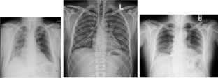
Machine learning and deep learning approach for medical image analysis: diagnosis to detection

Diagnosis of Pediatric Pneumonia with Ensemble of Deep Convolutional Neural Networks in Chest X-Ray Images

Convolutional neural networks: an overview and application in radiology

Data availability statement.

The data that support the findings of this study are openly available at https://web.nit.ac.ir/~y.baleghi/Emergency_COVID_Dataset.rar

World health organization (2020) Coronavirus disease 2019 (covid-19): situation report. Report No.: 94

Sethy PK, Behera SK (2020) Detection of coronavirus disease (covid-19) based on deep features

Elkorany AS, Elsharkawy ZF (2021) COVIDetection-Net: a tailored covid-19 detection from chest radiography images using deep learning. Optik 231:166405

Article   Google Scholar  

Corman VM et al (2020) Detection of 2019 novel coronavirus (2019-ncov) by real-time rt-pcr. Eurosurveillance 25(3):2000045

Kanne JP et al (2020) Essentials for radiologists on covid-19: an update–radiology scientific expert panel. Radiological Society of North America

Xie X et al (2020) Chest ct for typical coronavirus disease 2019 (covid-19) pneumonia: relationship to negative rt-pcr testing. Radiology 296(2):41–45

Qi X et al (2021) Chest x-ray image phase features for improved diagnosis of covid-19 using convolutional neural network. Int J Comput Assist Radiol Surg 16(2):197–206

Narin A, Kaya C, Pamuk Z (2021) Automatic detection of coronavirus disease (covid-19) using x-ray images and deep convolutional neural networks. Pattern Analysis and Applications, 1–14

Hemdan EE-D, Shouman MA, Karar ME (2020) Covidx-net: a framework of deep learning classifiers to diagnose covid-19 in x-ray images. arXiv preprint arXiv:2003.11055

Apostolopoulos ID, Mpesiana TA (2020) Covid-19: automatic detection from x-ray images utilizing transfer learning with convolutional neural networks. Physical and Engineering Sciences in Medicine 43(2):635–640

Brunese L et al (2020) Explainable deep learning for pulmonary disease and coronavirus covid-19 detection from x-rays. Comput Methods Programs Biomed 196:105608

Das D, Santosh K, Pal U (2020) Truncated inception net: covid-19 outbreak screening using chest x-rays. Physical and Engineering Sciences in Medicine 43(3):915–925

Panwar H et al (2020) Application of deep learning for fast detection of covid-19 in x-rays using ncovnet. Chaos, Solitons & Fractals 138:109944

Article   MathSciNet   Google Scholar  

Singh D, Kumar V, Kaur M (2020) Classification of covid-19 patients from chest ct images using multi-objective differential evolution-based convolutional neural networks. European Journal of Clinical Microbiology & Infectious Diseases 39(7):1379–1389

Ozturk T et al (2020) Automated detection of covid-19 cases using deep neural networks with x-ray images. Comput Biol Med 121:103792

Ucar F, Korkmaz D (2020) COVIDiagnosis-Net: deep bayes-squeezenet based diagnosis of the coronavirus disease 2019 (covid-19) from x-ray images. Med Hypotheses 140:109761

Li X, Li C, Zhu D (2020) COVID-MobileXpert: on-device covid-19 patient triage and follow-up using chest x-rays. IEEE

Elgendi M et al (2020) The performance of deep neural networks in differentiating chest x-rays of covid-19 patients from other bacterial and viral pneumonias. Front Med 7:550

Chandra TB et al (2021) Coronavirus disease (covid-19) detection in chest x-ray images using majority voting based classifier ensemble. Expert Syst Appl 165:113909

Khan W, Zaki N (2022) Covid-19 detection from chest x-ray using deep learning ensemble classifier. In: Data intelligence and cognitive informatics. Springer, ???, pp 429–441

Das AK et al (2021) Automatic covid-19 detection from x-ray images using ensemble learning with convolutional neural network. Pattern Anal Appl 24(3):1111–1124

Saha P, Sadi MS, Islam MM (2021) EMCNet: automated covid-19 diagnosis from x-ray images using convolutional neural network and ensemble of machine learning classifiers. Informatics in Medicine Unlocked 22:100505

Elgendi M et al (2020) COVID-19-Detection-using-chest-X-rays. https://github.com/Elgendi/COVID-19-Detection-Using-Chest-X-rays

Ahmad MS et al (2018) Evaluation of positioning errors for in routine chest x-ray at beit jala governmental hospital. Inernational J Chem. Pharamacy Technol 3(5):1–8

Google Scholar  

Myerburg MM et al (2010) AMPK agonists ameliorate sodium and fluid transport and inflammation in cystic fibrosis airway epithelial cells. Am J Respir Cell Mol Biol 42(6):676–684

Puddy E, Hill C (2007) Interpretation of the chest radiograph. Continuing Education in Anaesthesia, Critical Care & Pain 7(3):71–75

Schueler BA (1998) Clinical applications of basic x-ray physics principles. Radiographics 18(3):731–744

Faculty of veterinary medicine, Mansoura University, Egypt (2006). https://www.vetmansoura.com/archive/Radiology/ExposureFactors/Exposure3.html

Tompe A, Sargar K (2020) X-ray image quality assurance. StatPearls [Internet]

Barrett JF, Keat N (2004) Artifacts in ct: recognition and avoidance. Radiographics 24(6):1679–1691

Wu Y et al (2021) Image-based motion artifact reduction on liver dynamic contrast enhanced mri. bioRxiv

Cohen JP et al (2020) Covid-19 image data collection: Prospective predictions are the future. arXiv preprint arXiv:2006.11988

Mooney P (2020) Chest X-ray images (Pneumonia). https://www.kaggle.com/paultimothymooney/chest-xray-pneumonia/metadata

Atasever S et al (2022) A comprehensive survey of deep learning research on medical image analysis with focus on transfer learning. Clinical Imaging

Iandola FN et al (2016) Squeezenet: alexnet-level accuracy with 50x fewer parameters and< 0.5 mb model size

Redmon J (2013) Darknet: open source neural networks in C

Huang G et al (2017) Densely connected convolutional networks

Szegedy C et al (2015) Going deeper with convolutions

Szegedy C et al (2017) Inception-v4, inception-resnet and the impact of residual connections on learning

Xia X, Xu C, Nan B (2017) Inception-v3 for flower classification. In: 2017 2nd International conference on image, vision and computing (ICIVC). IEEE

Sandler M et al (2018) Mobilenetv2: inverted residuals and linear bottlenecks

Zoph B et al (2018) Learning transferable architectures for scalable image recognition

He K et al (2016) Deep residual learning for image recognition

Sagi O, Rokach L (2018) Ensemble learning: a survey. Wiley Interdisciplinary Reviews: Data Mining and Knowledge Discovery 8(4):1249

Huang F, Xie G, Xiao R (2009) Ensemble learning. IEEE

Ahemad MT, Hameed MA, Vankdothu R (2022) Covid-19 detection and classification for machine learning methods using human genomic data. Measurement: Sensors 24:100537

Dietterich TG (2002) Ensemble learning. The Handbook of Brain Theory and Neural Networks 2(1):110–125

Zargari Khuzani A, Heidari M, Shariati SA (2021) Covid-classifier: an automated machine learning model to assist in the diagnosis of covid-19 infection in chest x-ray images. Sci Rep 11(1):9887

Guhathakurata S, Kundu S, Chakraborty A, Banerjee JS (2021) A novel approach to predict covid-19 using support vector machine. In: Data science for COVID-19. Elsevier, ???, pp 351–364

Reddy RN (2020) Covid-19 detection using svm classifier. Engpaper Journal

Panwar H, Gupta P, Siddiqui MK, Morales-Menendez R, Bhardwaj P, Singh V (2020) A deep learning and grad-cam based color visualization approach for fast detection of covid-19 cases using chest x-ray and ct-scan images. Chaos, Solitons & Fractals 140:110190

Cheng Z, Liang J, Tao G, Liu D, Zhang X (2023) Adversarial training of self-supervised monocular depth estimation against physical-world attacks. arXiv preprint arXiv:2301.13487

Cheng Z, Liang J, Choi H, Tao G, Cao Z, Liu D, Zhang X (2022) Physical attack on monocular depth estimation with optimal adversarial patches. In: European conference on computer vision. Springer, pp 514–532

Cheng Z, Choi H, Liang J, Feng S, Tao G, Liu D, Zuzak M, Zhang X (2023) Fusion is not enough: single-modal attacks to compromise fusion models in autonomous driving. arXiv preprint arXiv:2304.14614

Wang W, Han C, Zhou T, Liu D (2022) Visual recognition with deep nearest centroids. arXiv preprint arXiv:2209.07383

Morteza Ghazali S, Alizadeh M, Mazloum J, Baleghi Y (2022) Modified binary salp swarm algorithm in eeg signal classification for epilepsy seizure detection. Biomed Signal Process Control 78:103858. https://doi.org/10.1016/j.bspc.2022.103858

Download references

Acknowledgements

We would like to thank Imam Khomeini Hospital of Fereydunkenar and Dr. Rahim Ebrahimi Jouibari, the previous head of the hospital, for providing the local dataset. We would also like to thank Mohammad Davoudi for examining the existing errors of the emergency dataset and Mehdi Navaei Moakhkhar for giving access to the workstation system for training deep neural networks.

This work has not received any funds.

Author information

Authors and affiliations.

Department of Electrical & Computer Engineering, University of Alberta, Edmonton, Alberta, Canada

Zahra Ebrahimi Jouibari & Hosein Navaei Moakhkhar

Department of Electrical & Computer Engineering, Babol Noshirvani University of Technology, Babol, Mazandaran, Iran

Yasser Baleghi

You can also search for this author in PubMed   Google Scholar

Corresponding author

Correspondence to Yasser Baleghi .

Ethics declarations

Conflict of interest.

The authors declare that they have no conflict of interest.

Ethical Approval

This article does not contain any studies with human participants or animals performed by any of the authors.

Additional information

Publisher's note.

Springer Nature remains neutral with regard to jurisdictional claims in published maps and institutional affiliations.

Rights and permissions

Springer Nature or its licensor (e.g. a society or other partner) holds exclusive rights to this article under a publishing agreement with the author(s) or other rightsholder(s); author self-archiving of the accepted manuscript version of this article is solely governed by the terms of such publishing agreement and applicable law.

Reprints and permissions

About this article

Jouibari, Z.E., Moakhkhar, H.N. & Baleghi, Y. Emergency COVID-19 detection from chest X-rays using deep neural networks and ensemble learning. Multimed Tools Appl (2023). https://doi.org/10.1007/s11042-023-17508-x

Download citation

Received : 10 May 2023

Revised : 17 September 2023

Accepted : 10 October 2023

Published : 08 November 2023

DOI : https://doi.org/10.1007/s11042-023-17508-x

Share this article

Anyone you share the following link with will be able to read this content:

Sorry, a shareable link is not currently available for this article.

Provided by the Springer Nature SharedIt content-sharing initiative

• Transfer learning
• Ensemble learning
• Deep neural network
• Chest X-ray
• Emergency condition

Advertisement

• Find a journal
• Publish with us
• Track your research

Help | Advanced Search

Computer Science > Machine Learning

Title: fundamentals of recurrent neural network (rnn) and long short-term memory (lstm) network.

Abstract: Because of their effectiveness in broad practical applications, LSTM networks have received a wealth of coverage in scientific journals, technical blogs, and implementation guides. However, in most articles, the inference formulas for the LSTM network and its parent, RNN, are stated axiomatically, while the training formulas are omitted altogether. In addition, the technique of "unrolling" an RNN is routinely presented without justification throughout the literature. The goal of this paper is to explain the essential RNN and LSTM fundamentals in a single document. Drawing from concepts in signal processing, we formally derive the canonical RNN formulation from differential equations. We then propose and prove a precise statement, which yields the RNN unrolling technique. We also review the difficulties with training the standard RNN and address them by transforming the RNN into the "Vanilla LSTM" network through a series of logical arguments. We provide all equations pertaining to the LSTM system together with detailed descriptions of its constituent entities. Albeit unconventional, our choice of notation and the method for presenting the LSTM system emphasizes ease of understanding. As part of the analysis, we identify new opportunities to enrich the LSTM system and incorporate these extensions into the Vanilla LSTM network, producing the most general LSTM variant to date. The target reader has already been exposed to RNNs and LSTM networks through numerous available resources and is open to an alternative pedagogical approach. A Machine Learning practitioner seeking guidance for implementing our new augmented LSTM model in software for experimentation and research will find the insights and derivations in this tutorial valuable as well.

Submission history

Access paper:.

• Other Formats

References & Citations

• Google Scholar
• Semantic Scholar

DBLP - CS Bibliography

Bibtex formatted citation.

Bibliographic and Citation Tools

Code, data and media associated with this article, recommenders and search tools.

• Institution

arXivLabs: experimental projects with community collaborators

arXivLabs is a framework that allows collaborators to develop and share new arXiv features directly on our website.

Both individuals and organizations that work with arXivLabs have embraced and accepted our values of openness, community, excellence, and user data privacy. arXiv is committed to these values and only works with partners that adhere to them.

Have an idea for a project that will add value for arXiv's community? Learn more about arXivLabs .

Main Navigation

• Contact NeurIPS
• Code of Ethics
• Code of Conduct
• Create Profile
• Journal To Conference Track
• Diversity & Inclusion
• Proceedings
• Future Meetings
• Exhibitor Information
• Privacy Policy

NeurIPS 2024, the Thirty-eighth Annual Conference on Neural Information Processing Systems, will be held at the Vancouver Convention Center

Monday Dec 9 through Sunday Dec 15. Monday is an industry expo.

Registration

Pricing » Registration 2024 Registration Cancellation Policy » . Certificate of Attendance

Our Hotel Reservation page is currently under construction and will be released shortly. NeurIPS has contracted Hotel guest rooms for the Conference at group pricing, requiring reservations only through this page. Please do not make room reservations through any other channel, as it only impedes us from putting on the best Conference for you. We thank you for your assistance in helping us protect the NeurIPS conference.

Announcements

• The call for High School Projects has been released
• The Call For Papers has been released
• See the Visa Information page for changes to the visa process for 2024.

Latest NeurIPS Blog Entries [ All Entries ]

Important dates.

If you have questions about supporting the conference, please contact us .

View NeurIPS 2024 exhibitors » Become an 2024 Exhibitor Exhibitor Info »

Organizing Committee

General chair, program chair, workshop chair, workshop chair assistant, tutorial chair, competition chair, data and benchmark chair, diversity, inclusion and accessibility chair, affinity chair, ethics review chair, communication chair, social chair, journal chair, creative ai chair, workflow manager, logistics and it, mission statement.

The Neural Information Processing Systems Foundation is a non-profit corporation whose purpose is to foster the exchange of research advances in Artificial Intelligence and Machine Learning, principally by hosting an annual interdisciplinary academic conference with the highest ethical standards for a diverse and inclusive community.

About the Conference

The conference was founded in 1987 and is now a multi-track interdisciplinary annual meeting that includes invited talks, demonstrations, symposia, and oral and poster presentations of refereed papers. Along with the conference is a professional exposition focusing on machine learning in practice, a series of tutorials, and topical workshops that provide a less formal setting for the exchange of ideas.

More about the Neural Information Processing Systems foundation »